Electromagnetic waves in vacuum
Fondamental : Fundamental d'Alembert's propagation equation
A distribution (D) of charges localized around a point O, whose densities depend on time (example : a metal antenna).
According to Maxwell-Gauss' equation and Maxwell-Ampere's equation, this distribution (D) is the source of \(\vec E\) and \(\vec B\) fields variables in time that will be created in the vicinity of O.
A point M in this vicinity, although located outside (D), is itself a source of fields because of the terms \(\partial \vec B/\partial t\) and \(\partial \vec E /\partial t\) "from O" that play a role of sources in Maxwell-Faraday 's equation and Maxwell-Ampere's equation.
Points P in the vicinity of M are in turn in their own vicinities sources of variable fields in time ...
Thus understood that the electromagnetic field propagates being reminiscent of wrinkles that is transmitted from point to point on the surface of the water.
"The coupling which is introduced into the Maxwell equations by the presence of the two partial derivatives with respect to time \(\partial \vec B/\partial t\) and \(\partial \vec E /\partial t\) is the origin of the propagation phenomenon of the electromagnetic field".
Obtaining the propagation equations of electromagnetic field :
We calculate the curl of the Maxwell-Faraday equation :
\(\overrightarrow {rot} \left( {\overrightarrow {rot} \;\vec E} \right) = - \frac{\partial }{{\partial t}}\left( {\overrightarrow {rot\;} \vec B} \right)\;\;\)
Or :
\(\overrightarrow {rot} \left( {\overrightarrow {rot} \;\vec E} \right) = \overrightarrow {grad} \left( {div\;\vec E} \right) - \Delta \vec E\;\;\;\)
With :
\(div\;\vec E = \frac{\rho }{{{\varepsilon _0}}}\;and\;\overrightarrow {rot} \;\vec B = {\mu _0}\vec j + {\varepsilon _0}{\mu _0}\frac{{\partial \vec E}}{{\partial t}}\)
It comes :
\(\overrightarrow {grad} \left( {\frac{\rho }{{{\varepsilon _0}}}} \right) - \Delta \vec E\;\; = - \frac{\partial }{{\partial t}}\left( {{\mu _0}\vec j + {\varepsilon _0}{\mu _0}\frac{{\partial \vec E}}{{\partial t}}} \right)\)
Or, finally :
\(\Delta \vec E - {\varepsilon _0}{\mu _0}\frac{{{\partial ^2}\vec E}}{{\partial {t^2}}} = \frac{1}{{{\varepsilon _0}}}\overrightarrow {grad} \;\rho + {\mu _0}\frac{{\partial \vec j}}{{\partial t}}\)
Symmetrically, \(\vec E\) is eliminated in favor of \(\vec B\) by calculating the curl of Maxwell Ampere's equation :
\(\overrightarrow {rot} \left( {\overrightarrow {rot} \;\vec B} \right) = \overrightarrow {grad} \left( {div\;\vec B} \right) - \Delta \vec B = {\mu _0}\overrightarrow {rot} \;\vec j + {\varepsilon _0}{\mu _0}\frac{\partial }{{\partial t}}\left( {\overrightarrow {rot} \;\vec E} \right)\;\;\)
So :
\(\overrightarrow {grad} \left( 0 \right) - \Delta \vec B = {\mu _0}\overrightarrow {rot} \;\vec j + {\varepsilon _0}{\mu _0}\frac{\partial }{{\partial t}}\left( { - \frac{{\partial \vec B}}{{\partial t}}} \right)\;\;\)
Finally :
\(\Delta \vec B - {\varepsilon _0}{\mu _0}\frac{{{\partial ^2}\vec B}}{{\partial {t^2}}} = - {\mu _0}\overrightarrow {rot} \;\vec j\)
Attention : D'Alembert's propagation equation in vaccum
In an area with neither charges nor currents (\(\rho=0\) and \(\vec j=\vec 0\)) :
\(\Delta \vec E - {\varepsilon _0}{\mu _0}\frac{{{\partial ^2}\vec E}}{{\partial {t^2}}} = \vec 0\;\;\;\;\;\;\;and\;\;\;\;\;\;\;\Delta \vec B - {\varepsilon _0}{\mu _0}\frac{{{\partial ^2}\vec B}}{{\partial {t^2}}} = \vec 0\)
This is d'Alembert's equation (classical equation of wave propagation, also known equation of vibrating strings) established in the eighteenth century to model the vibrations of a stretched string (see the lesson "Waves in a string").
Solutions of this equation reflect a phenomenon of speed of propagation \(c\) (speed of light in vacuum) :
\(c=\frac{1}{\sqrt{\varepsilon_0 \mu_0}}\)
Fondamental : Solution of the d'Alembert equation in the form of traveling wave
In one dimension, the d'Alembert's equation is written :
\(\frac{\partial^2s(z,t)}{\partial z^2} - {\varepsilon _0}{\mu _0}\frac{{{\partial ^2}s(z,t)}}{{\partial {t^2}}} = 0\;\;\;\;\;so\;\;\;\;\;\frac{\partial^2s(z,t)}{\partial z^2} - \frac{1}{{{c^2}}}\frac{{{\partial ^2}s(z,t)}}{{\partial {t^2}}} = 0\;\;\;\;(\frac{1}{{{c^2}}} = {\varepsilon _0}{\mu _0})\)
Where \(s(z,t)\) represents the coordinates of the electromagnetic field, and as a function only of \(z\) and \(t\).
It is shown that the form of the solution of the d'Alembert's wave equation is written as :
\(s(z,t) = f(t - \frac{z}{c}) + g(t + \frac{z}{c})\)
Where \(f\) is an arbitrary function of the variable \( (t-z/c)\) and \(g\) a function of the variable \(( t+z/c)\).
Physical interpretation :
Considering a function of the form :
\({s_ + }(z,t) = f(t - \frac{z}{c})\)
It is found that :
\(f(t - \frac{z}{c}) = f(t + \Delta t - \frac{{z + \Delta z}}{c})\)
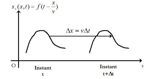
For every pair \(\Delta z\) and \(\Delta t\) satisfying :
\(\Delta z=c\Delta t\)
So \(s_+(z,t)\) represents a signal which propagates without deformation at speed \(c\) along the axis (Oz) in the positive direction.
The solution :
\({s_ - }(z,t) = f(t + \frac{z}{c})\)
Represents a signal which propagates without deformation at speed \(c\) along the axis (Oz) in the negative direction.
In a plane \(z=cste\), functions \({s_ + }(z,t) = f(t - \frac{z}{c})\) and \({s_ - }(z,t) = f(t + \frac{z}{c})\) take, at all times, the same value : we talk about plane waves and the plans \(z=cste\) are called wave plans.
A source (for example, a radio station) transmits a priori spherical waves ; however, at a great distance from there, the received wave may be locally treated to a progressive plane wave.
Monochromatic progressive plane waves (or harmonics, MPPW) :
The wave equation is linear ; therefore, the Fourier analysis to suggest that any solution of this equation is the sum of sinusoidal functions of time.
We limit ourselves here to harmonic solutions of the d'Alembert's equation, that is to say the form of solutions (for a wave propagating in the direction \(x>0\)) :
\(s(z,t) = A\;\cos \left( {\omega (t - \frac{z}{c})} \right)\)
These solutions correspond to harmonic progressive plane waves (HPPW or MPPW).
These functions, in time period \(T=2\pi/\omega\) have a spatial period \(\lambda=cT\) called wavelength.
We define the wave vector \(\vec k\) such that :
\(\vec k = k\;{\vec u_z}\;\;\;\;\;\;\;\;\;\;with\;\;\;\;\;\;\;\;\;\;k = \frac{\omega }{c} = \frac{{2\pi }}{\lambda }\)
HPPW is then of the form :
\(s(z,t) = A\;\cos \left( {\omega t - kz} \right)\)

In real notation, the electric field can be written :
\(\vec E(z,t) = {\vec E_0}\cos (\omega (t - \frac{z}{c})) = {\vec E_0}\cos (\omega t - kz)\)
In complex notation, we note the electromagnetic field in the form :
\(\underline {\vec E} (z,t) = {\underline {\vec E} _0}\;{e^{i(\omega t - kz)}}\;\;\;\;\;and\;\;\;\;\;\underline {\vec B}( z,t) = {\underline {\vec B} _0}\;{e^{i(\omega t - kz)}}\)
If there is any direction of the wave, in the direction of the unit vector \(\vec u\) :
\(\underline {\vec E} (x,y,z,t) = {\underline {\vec E} _0}\;{e^{i(\omega t - \vec k.\vec r)}}\;\;\;\;\;and\;\;\;\;\;\underline {\vec B}( x,y,z,t) = {\underline {\vec B} _0}\;{e^{i(\omega t - \vec k.\vec r)}}\)
Where \(\vec k = k \;\vec u\) (\(\vec u\) unit vector indicating the direction of propagation) is the wave vector and \(\vec r = \vec {OM}\) (O, the origin of the frame of reference and M the point of observation).
Méthode : The vector operators for HPPW in complex notation
Take into account the choice of the complex notation, the vector operators are simplified.
With :
\(\vec E = {\vec E_0}\exp (i(\omega t - \vec k.\vec r)) = {\vec E_0}\exp (i(\omega t - {k_x}x - {k_y}y - {k_z}z))\)
It comes :
\(div\;\underline {\vec E} = \frac{{\partial {{\underline E }_x}}}{{\partial x}} + \frac{{\partial {{\underline E }_y}}}{{\partial y}} + \frac{{\partial {{\underline E }_z}}}{{\partial z}} = - i{k_x}{\underline E _x} - i{k_y}{\underline E _y} - i{k_z}{\underline E _z} = - i\;\vec k.\underline {\vec E}\)
The same :
\(\overrightarrow {rot} \;\underline {\vec E} = - i\;\vec k \wedge \underline {\vec E} \;\;\;\;\;\;\;\;\;\;and\;\;\;\;\;\;\;\;\;\;\Delta \underline {\vec E} = - {k^2}\underline {\vec E}\)
Finally we can notice that the "nabla operator" is equivalent to :
\(\vec \nabla = -i\vec k\)
The four Maxwell equations then become :
\(div\;\underline {\vec E} = - i\;\vec k.\underline {\vec E} = 0\;\;\;\;;\;\;\;\;div\;\underline {\vec B} = - i\;\vec k.\underline {\vec B} = 0\)
And :
\(\overrightarrow {rot} \;\underline {\vec E} = - i\;\vec k \wedge \underline {\vec E} = - (i\omega \underline {\vec B} )\;\;\;\;;\;\;\;\;\overrightarrow {rot} \;\underline {\vec B} = - i\;\vec k \wedge \underline {\vec B} = \frac{1}{{{c^2}}}(i\omega \underline {\vec E} )\)
Fondamental : Structure of the electromagnetic field in vacuum
Previously written Maxwell's equations give for example :
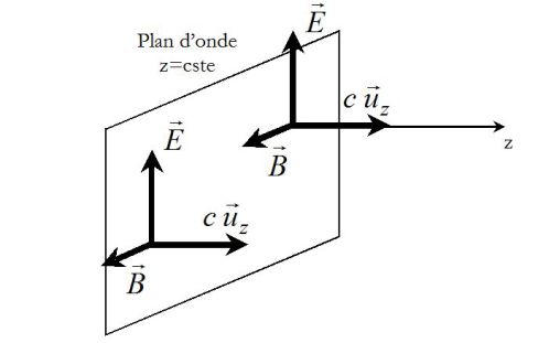
\(\vec k.\underline {\vec E} = 0\;\;\;\;\;\;\;and\;\;\;\;\;\;\;\vec k.\underline {\vec B} = 0\;\)
Thus, the coordinates of the electromagnetic field parallel to the propagation direction are zero : the electromagnetic field is transverse.
We also obtain from the Maxwell-Faraday equation :
\(\underline {\vec B} = \frac{{\vec k}}{\omega } \wedge \underline {\vec E} = \frac{1}{c}\vec u \wedge \underline {\vec E}\)
Finally, the electromagnetic fields of a progressive plane wave are orthogonal to the propagation direction and orthogonal to each other.
the triad \((\vec E,\vec B,\vec c=c\vec u)\) is direct and \(E=Bc\).
Important notes :
The structural relationship of a plane wave :
\(\underline {\vec B} = \frac{{\vec k}}{\omega } \wedge \underline {\vec E} = \frac{1}{c}\vec u \wedge \underline {\vec E}\)
is obviously checked only by harmonic monochromatic plane waves.
In particular, when the amplitude of the wave will depends on the space coordinates \(x\) or \(y\), the relationship between the field \(\vec E\) and the field \(\vec B\) will be different.
Lorentz force :
The force exerted by the electromagnetic wave on a particle of charge \(q\) and velocity \(\vec v\) is :
\(\vec f = q\;\vec E + q\;\vec v \wedge \vec B = {\vec f_e} + {\vec f_m}\)
Therefore, the ratio of the electric force to the magnetic force is :
\(\frac{{{f_e}}}{{{f_m}}} = \frac{E}{{vB}} = \frac{c}{v}\)
Therefore, for a non-relativistic particle (\(v<<c\)), the magnetic force is negligible with respect to the electric force.
Complément : Lecture videos on radiocommunications

Fondamental : The propagation of energy
The following results are valid for a progressive plane wave, not necessarily sinusoidal (or harmonic).
The energy density \(u_{em}\) for a progressive plane wave is :
\({u_{em}} = \frac{1}{2}{\varepsilon _0}{\vec E\;^2} + \frac{1}{{2{\mu _0}}}{\vec B}\;^2\)
Considering \(E=Bc\), it comes (using \(c=1/\sqrt{\varepsilon_0 \mu_0}\)) :
\({u_{em}} = {\varepsilon _0}{\vec E\;^2} = \frac{1}{{{\mu _0}}}{\vec B\;^2}\)
Note that there is equipartition of electric and magnetic contributions to the energy density.
The Poynting vector is :
\(\vec \Pi = \frac{{\vec E \wedge \vec B}}{{{\mu _0}}}\)
Either, with \(\vec B = \frac{{{{\vec u}_z}}}{c} \wedge \vec E\) :
\(\vec \Pi = \frac{1}{{c{\mu _0}}}\vec E \wedge ({\vec u_z} \wedge \vec E) = \frac{1}{{c{\mu _0}}}{\vec E\;^2}\;{\vec u_z}\;\;\;\;\;\;\;\;\;\;(with\;\vec E.\;{\vec u_z} = 0)\)
Finally :
\(\vec \Pi = {\varepsilon _0}c\;{\vec E\;^2}\;{\vec u_z} = c{u_{em}}\;{\vec u_z}\)
The Poynting vector is collinear to the direction of propagation ; if we return to the definition of the current density vector :
\(\vec j = \rho \vec v\)
corresponding to an ensemble movement of charge of density \(\rho\) at speed \(\vec v\), we find that the relationship \(\vec \Pi = c{u_{em}}\;{\vec u_z}\) simply expresses the progressive plane electromagnetic wave in vacuum transports energy in its own propagation direction and with a speed equal to its speed \(c\) (\({\vec v_{em}} = \vec \Pi /{u_{EM}} = c{\vec u_z}\)).
Note (energy propagation velocity) :
This result can be found by considering the cylinder of cross-section (S) and of length \(v_{em}dt\) parallel to propagation direction.
The energy that goes through this area during \(dt\) is \(u_{em}v_{em}Sdt\).
It is also equal to the flux of the Poynting vector (times \(dt\)) :
\({u_{em}}{v_{em}}Sdt = \Pi\; Sdt\;\;\;\;\;\;\;so\;\;\;\;\;\;\;{v_{em}} = \frac{\Pi }{{{u_{em}}}} = c\)
The energy propagation velocity is equal to \(c\).
Average Poynting vector and average power received by a detector :
Electromagnetic waves usually have high frequencies.
The detectors are often sensitive only to temporal average values of the power they receive.
Thus, the average power received by a detector whose surface \(S\) is perpendicular to the direction of propagation is :
\({P_m} = \left\langle {\vec \Pi } \right\rangle .\;S\;{\vec u_z} = \left\langle \Pi \right\rangle .S\)
Where \(\left\langle \Pi \right\rangle\) denotes the average algebric value of the Poynting vector, equal to :
\(\left\langle \Pi \right\rangle = {\varepsilon _0}c\;\left\langle {{E^2}} \right\rangle\)
For an electric field of the form :
\(E = {E_0}\cos (\omega t - \vec k.\vec r - {\phi _0})\)
\(\left\langle {{E^2}} \right\rangle = \frac{{E_0^2}}{2}\)
And so :
\(\left\langle \Pi \right\rangle = {\varepsilon _0}c\frac{{\;E_0^2}}{2}\)
Using the complex notation for the power :
If \(\underline f\) and \(\underline g\) are two sinusoidal functions in complex notation, while the average of the product \(fg\) is :
\(\left\langle {fg} \right\rangle = \frac{1}{2}{\mathop{\rm Re}\nolimits} (\underline f .\underline {g}^*)\)
Where \(\underline g^*\) is the conjugate of \(\underline g\).
We can apply this formula to calculate the average power in electricity :
\(P = \left\langle {ui} \right\rangle = \frac{1}{2}{\mathop{\rm Re}\nolimits} (\underline u .{\underline i ^*}) = \frac{1}{2}{U_m}{I_m}\cos \phi = {U_e}{I_e}\cos \phi\)
The average value of the electromagnetic energy density is then :
\(\left\langle {{e_{em}}} \right\rangle = \frac{1}{2}\left( {{\varepsilon _0}\frac{1}{2}{\mathop{\rm Re}\nolimits} (\underline {\vec E} .{{\underline {\vec E} }^*}) + \frac{1}{{{\mu _0}}}\frac{1}{2}{\mathop{\rm Re}\nolimits} (\underline {\vec B} .{{\underline {\vec B} }^*})} \right)\)
Either :
\(\left\langle {{e_{em}}} \right\rangle = \frac{1}{2}\left( {\frac{1}{2}{\varepsilon _0}E_0^2 + \frac{1}{{2{\mu _0}}}B_0^2} \right) = \frac{1}{2}{\varepsilon _0}E_0^2\)
The average value of the Poynting vector is calculated in the same way :
\(\left\langle {\vec \Pi } \right\rangle = \frac{1}{2}{\mathop{\rm Re}\nolimits} (\frac{1}{{{\mu _0}}}\underline {\vec E} \wedge {\underline {\vec B} \;^*}) = \frac{1}{{2{\mu _0}}}{\mathop{\rm Re}\nolimits} (\underline {\vec E} \wedge (\frac{{\vec u}}{c} \wedge {\underline {\vec E}\; ^*}))\)
Either :
\(\left\langle {\vec \Pi } \right\rangle = \frac{1}{{2c{\mu _0}}}{\mathop{\rm Re}\nolimits} (\underline {\vec E} .{\underline {\vec E} ^*}\vec u - \underline {\vec E} .\vec u\;{\underline {\vec E} ^*}) = \frac{1}{2}{\varepsilon _0}cE_0^2\;\vec u\)
Some figures :
Amplitudes of the electromagnetic field of a laser beam :
A helium-neon laser emits a cylinder beam of cross section \(1\;mm^2\) and power \(1\;mW\).
It produces a linearly polarized wave.
Determine the amplitude of electromagnetic fields.
The sine wave is sinusoidal quasi-plane.
Electromagnetic fields are equal to :
\({E_0} = \sqrt {\frac{{2{\mu _0}cP}}{S}} = {8,7.10^2}\;V.{m^{ - 1}}\;\;\;\;\;\;\;;\;\;\;\;\;\;\;{B_0} = \frac{{{E_0}}}{c} = {2,9.10^{ - 6}}\;T\)
Diffusion from a radio station :
A monochromatic wave source (E) in a plain emits linearly polarized isotropic radiation of a power of \(1\; MW\).
Calculating the magnitude of the electric field at a distance \(r\) and \(1\; 000\; km\).
We find :
\({E_0} = \sqrt {\frac{{{\mu _0}cP}}{\pi }} \frac{1}{r} = {1,1.10^4}\frac{1}{r}\;V.{m^{ - 1}}\;\;\;\;\;\;\;\;\;\;({1,1.10^{ - 2}}\;V.{m^{ - 1}}\;for\;1\;000\;km)\)
Complément : Solution of the d'Alembert's equation in the form of standing wave
We look for solutions of the d'Alembert's equation of the form ( variables separation method) :
\(s(z,t) = f(z)\;g(t)\)
Substituting in the d'Alembert's equation :
\(\frac{{{\partial ^2}s(z,t)}}{{\partial {z^2}}} - \frac{1}{{{c^2}}}\frac{{{\partial ^2}s(z,t)}}{{\partial {t^2}}} = 0\)
It becomes :
\(f"(z)g(t) - \frac{1}{{{c^2}}}f(z)\ddot g(t) = 0\)
Where :
\(\frac{1}{{f(z)}}f"(z) = \frac{1}{{{c^2}}}\frac{{\ddot g(t)}}{{g(t)}} = cste = K\)
This produces two differential equations :
\(\frac{1}{{f(z)}}f''(z) = K\;\;\;\;\;\;\;\;\;\;and\;\;\;\;\;\;\;\;\;\;\;\frac{1}{{{c^2}}}\frac{{\ddot g(t)}}{{g(t)}} = K\)
Or again :
\(f''(z) - Kf(z) = 0\;\;\;\;\;\;\;\;\;\;and\;\;\;\;\;\;\;\;\;\ddot g(t) - {c^2}Kg(t) = 0\)
If \(K>0\), the solution of the second differential equation is of the form :
\(g(t) = A{e^{c\sqrt K \;t}} + B{e^{ - c\sqrt K \;t}}\)
This solution is rejected : indeed, it is either a divergent solution or a transitional solution.
In the following, it is assumed \(K<0\) ; then, by denoting \(- {c^2}K = {\omega ^2}\) :
\(g(t) = A\;cos (\omega t - \phi )\)
The first equation then gives :
\(f''(z) + \frac{{{\omega ^2}}}{{{c^2}}}f(z) = 0\;\;\;\;\;\;so\;\;\;\;\;f(z) = B\;cos \left( {\frac{\omega }{c}z - \psi } \right)\)
Thus, the global solution of the d'Alembert's equation is :
\(s(z,t) = C\;cos \left( {\frac{\omega }{c}z - \psi } \right)\;\cos \left( {\omega t - \phi } \right)\)
We denote in the following \(k=\omega/c\), then :
\(s(z,t) = C\;cos \left( {kz - \psi } \right)\;\cos \left( {\omega t - \phi } \right)\)
This type of solutions, called standing plane waves is very different from a progressive plane wave : spatial and temporal dependencies occur separately ; spatial dependence occurs in the amplitude of the temporal oscillation and no longer in phase, so that all points vibrate in phase or in phase opposition.
The shape of a rope (for instance, see lesson "Waves in a string") at different instants is shown in the following figure.
Some points of the rope are fixed and are called nodes of vibrations ; others have a maximum vibration amplitude and are called anti-nodes vibrations.
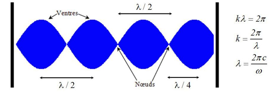
The distance between two successive nodes is equal to \(\lambda/2\).
The distance between two successive anti-nodes is equal to \(\lambda/2\).
The distance between a node and a successive anti-node equals \(\lambda/4\).