Fourier analysis and electronic
Fondamental : Fourier series decomposition
A periodic signal \(s(t)\) of period \(T\) may (under certain conditions that are supposed to be checked physically) be decomposed into a sum of sine functions (Fourier series decomposition) :
\(s(t) = {a_0} + \sum\limits_{n = 1}^\infty {({a_n}\cos (n\omega t )+ {b_n}\sin( n\omega t))\;\;\;\;\;\;\;(n\;integer\;and\;\omega = \frac{{2\pi }}{T})}\)
The coefficients \(a_0\), \(a_n\) and \(b_n\) are constant and given by the integrals :
\(a_0=\frac{1}{T} \int_0^Ts(t)dt\;\;\;\;\; ;\;\;\;\;\;a_n=\frac{2}{T} \int_0^Ts(t)cos(n\omega t)dt\;\;\;\;\; ;\;\;\;\;\;b_n=\frac{2}{T} \int_0^Ts(t)sin(n\omega t)dt\)
We note that the coefficient \(a_0\) is the average value of \(s(t)\).
The term corresponding to \(n=1\) (an angular frequency equal to that of the signal \(s(t)\)) :
\(a_1cos\omega t +b_1sin\omega t\)
is called the fundamental.
The general term :
\(a_ncos(n\omega t) +b_nsin(n\omega t)\)
is harmonic of rang \(n\).
Even signal \(s(t)\) and odd signal :
If \(s(t)\) is odd (\(s(-t)=-s(t))\) :
The development in Fourier series of the signal \(s(t)\) then includes only sine terms (coefficients \(a_n\) are zero) :
\(s(t) = \sum\limits_{n = 1}^\infty { b_n} sin( n\omega t)\)
If \(s(t)\) is even (\(s(-t)=s(t))\) :
The development in Fourier series of the signal \(s(t)\) then includes only cosine terms (coefficients \(b_n\) are zero) :
\(s(t) = \sum\limits_{n = 1}^\infty { a_n} cos( n\omega t)\)
Frequency spectrum :
The general term \(a_ncos(n\omega t) +b_nsin(n\omega t)\) may be in the form :
\({a_n}\cos (n\omega t) + {b_n}\sin (n\omega t) = \sqrt {a_n^2 + b_n^2} \left[ {\frac{{{a_n}}}{{\sqrt {a_n^2 + b_n^2} }}\cos (n\omega t) + \frac{{{b_n}}}{{\sqrt {a_n^2 + b_n^2} }}\sin (n\omega t)} \right]\)
If we denote :
\({c_n} = \sqrt {a_n^2 + b_n^2} \;\;\;\;\;;\;\;\;\;\;\tan {\varphi _n} = \frac{{{b_n}}}{{{a_n}}}\;\;\;\;\;;\;\;\;\;\;\cos {\varphi _n} = \frac{{{a_n}}}{{\sqrt {a_n^2 + b_n^2} }}\)
So :
\(a_ncos(n\omega t) +b_nsin(n\omega t)=c_n cos(n\omega t -\varphi_n)\)
And the periodic signal \(s(t)\) becomes :
\(s(t)=\sum\limits_{n = 1}^\infty c_n cos(n\omega t -\varphi_n)\)
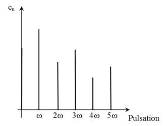
The frequency spectrum (or spectral representation) of the signal \(s(t)\) is obtained by taking the ordinate the amplitude of the harmonics (that is to say the coefficients \(a_n\), \(b_n\) or \(c_n\)) and in the abscissa the corresponding pulses.
Exemple : Some special signals
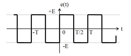
Square wave :
The niche voltage (or square voltage) \(e(t)\) in the following figure can be decomposed into Fourier series as :
\(e(t) = \frac{{4E}}{\pi }\left[ {\sin \omega t + \frac{1}{3}\sin 3\omega t + \frac{1}{5}\sin 5\omega t + ...} \right]\)
This is an odd function. Therefore, the development in Fourier series does not comprise cosine terms.
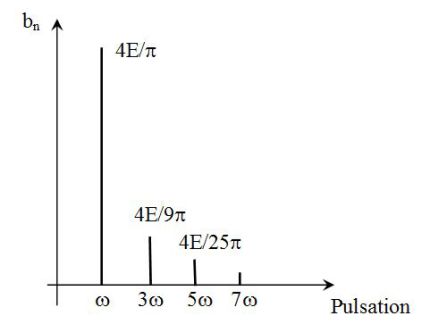
Note that the harmonics are odd rang (of form \(n=2p+1\)) and that the coefficients \(b_n\) decrease as \(1/n\).
The following figure shows the frequency spectrum of the square signal.

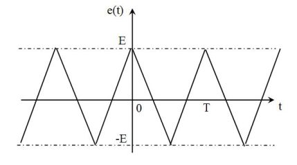
Triangular signal :
The triangular voltage \(e(t)\) of the figure can be written :
\(e(t) = \frac{{8E}}{\pi^2 }\left[ {\cos \omega t + \frac{1}{3^2}\cos 3\omega t + \frac{1}{5^2}\cos 5\omega t + ...} \right]\)
This is an even function. Therefore, the development in Fourier series does not include the sine terms.
Note that the harmonics are odd (of form \(n=2p+1\)) and that the coefficients \(a_n\) decrease as \(1/n^2\).
The following figure shows the frequency spectrum of the square signal.
Complément : Average value, effective (RMS) value, Parseval formula and form factor of a signal
\(s(t)\) is a periodic signal, the Fourier series decomposition is :
\(s(t) = {a_0} + \sum\limits_{n = 1}^\infty {{c_n}\cos (n\omega t - {\varphi _n})}\)
The average value of \(s(t)\) is :
\({S_{moy}} = \left\langle {s(t)} \right\rangle = \frac{1}{T}\int_0^T {s(t)dt} = {a_0}\)
The RMS value is :
\({S_{eff}} = \sqrt {\left\langle {{s^2}(t)} \right\rangle } = \sqrt {\frac{1}{T}\int_0^T {{s^2}(t)dt} }\)
Using the decomposition into Fourier series :
\({S_{eff}}^2 = \frac{1}{T}\int_0^T {{{\left[ {{a_0} + \sum\limits_{n = 1}^\infty {{c_n}\cos (n\omega t - {\varphi _n})} } \right]}^2}dt}\)
Knowing that the average value of a sine function is zero, the average value of a product of two sinusoidal functions of different pulses is zero and that the average value of the sine square is \(1/2\), we get :
\({S_{eff}}^2 = {a_0}^2 + \sum\limits_{n = 1}^\infty {\frac{{{c_n}^2}}{2}}\)
This is the formula Parseval : "The square of the effective (RMS) value of a periodic signal is equal to the sum of the square of its mean value and squares of the RMS values of the harmonics".
Two special cases :
If \(s(t)\) is a pure sine wave :
\({S_{eff}} = \frac{{{S_{\max }}}}{{\sqrt 2 }}\)
If a sinusoidal signal \(s(t)\) is shifted by a DC component \(a_0\) :
\({S_{eff}} = \sqrt {{a_0}^2 + \frac{{{S_{max}}^2}}{2}}\)
The form factor (noted \(f\)) of a periodic signal \(s(t)\) is the ratio of the RMS value and average value of the signal :
\(f = \frac{{{S_{eff}}}}{{{S_{moy}}}} = \frac{{\sqrt {{a_0}^2 + \frac{1}{2}\sum\limits_{n = 1}^\infty {{c_n}^2} } }}{{{a_0}}}\)
For continuous signal : \(f=1\).
\(f\) is not defined for a periodic signal of zero mean value.
For a sinusoidal-wave rectified signal :
\(f = \frac{\pi }{{2\sqrt 2 }} \approx 1,11\)

Complément : Harmonic Distortion
Consider a nonlinear electrical system when the input voltage is sinusoidal, the output voltage is not or has a different pulse to that of the input.
Is then carried out a harmonic decomposition of the output signal (assuming that it is periodic) :
\(s(t) = {a_0} + \sum\limits_{n = 1}^\infty {({a_n}\cos (n\omega t) + {b_n}\sin (n\omega t))}\)
If the system was strictly linear, only \(1\) degree coefficients are nonzero.
Terms of order greater than or equal to \(2\) are the harmonic distortion.
Called harmonic distortion rate, noted \(\tau\) and expressed in dB, the ratio between the power of the harmonic terms and that of the total signal :
\(\tau = 10\log \left[ {\frac{{\sum\limits_{k = 2}^\infty {(a_k^2 + b_k^2)} }}{{\sum\limits_{k = 1}^\infty {(a_k^2 + b_k^2)} }}} \right]\)
For a linear system, \(\tau\) tends to \(-\infty\).
Example :
The output is connected to the input by the relationship :
\(s = {s_0} + a\;e + b\;{e^2} + c\;{e^3}\)
With :
\({s_0} = 0,1\;V\;;\;a = 10\;;\;b = 0,1\;{V^{ - 1}}\;and\;\;c = 0,01\;{V^{ - 2}}\;\;(and\; - 1\;V \le e \le 1\;V)\)
The sinusoidal input is assumed :
\(e(t) = E\cos \omega t\)
The output is :
\(s = {s_0} + a\;(E\cos \omega t) + b\;{(E\cos \omega t)^2} + c\;{(E\cos \omega t)^3}\)
With :
\({\cos ^2}\omega t = \frac{{1 + \cos (2\omega t)}}{2}\;\;\;\;\;and\;\;\;\;\;{\cos ^3}\omega t = \frac{{\cos (3\omega t) + 3\cos \omega t}}{4}\)
It comes :
\(s(t) = {s_0} + b\frac{{{E^2}}}{2} + \left( {aE + \frac{3}{4}c{E^3}} \right)\cos \omega t + b\frac{{{E^2}}}{2}\cos 2\omega t + \frac{1}{4}c{E^3}\cos 3\omega t\)
Assuming \(E=1\;V\), we obtain :
\(s(t) = 0,15 + 10\cos \omega t + 0,05\cos 2\omega t + 0,0025\cos 3\omega t\)
Harmonic distortion rate is :
\(\tau = - 46\;dB\)
Harmonic analysis (using a spectrum analyzer, for example) would bring out these nonlinearities.