Quantum tunneling microscope
Take 15 minutes to prepare this exercise.
Then, if you lack ideas to begin, look at the given clue and start searching for the solution.
A detailed solution is then proposed to you.
If you have more questions, feel free to ask them on the forum.
A document about quantum tunneling microscope.
Question
Give, in a few words, and by using the picture, the principle of the quantum tunneling microscope.
Do you know other phenomena where quantum tunneling microscope effect appears ?

Solution
To simplify, a sensor (tip or probe) follows the surface of the object.
The sensors sweeps or scans the studied surface. A computer adjusts (via a subservience service) in real-time the height of the sensor to maintain a constant current (tunneling current) and registers this height to recreate the surface.
In order to do so, a conductive tip is placed in front of the surface to study with a positioning system of great precision (realized with the help of piezoelectricity).
The current resulting to the passage of electrons between the surface and the sensors, by quantum tunneling can be measured : the free electrons of the metal hardly come out to the surface so if the sensor approaches them really closely but without touching them, an electric current can be registered.
In most cases, the current decreases very rapidly -exponentially- in function of the distance separating the surface from the sensor, with a characteristic distance of a few dozen of nanometers.
When the sensor above the sample is set in motion with a movement of sweeping, the height of the latter is adjusted in order to conserve a constant intensity of tunneling current, thanks to a retroaction buckle.
The profile of the surface can thus be determined with a precision inferior to the inter-atomic distances.
Question
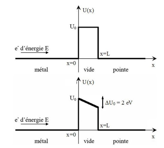
A potential barrier \(U(x)\) exists between the explorer sensor and the metallic sample.
It is modeled as shown on the picture, with \(L=1\) \(nm\) and \(U_0=6\) \(eV\).
An electron arrives on the potential barrier.
Its energy is \(E=1\) \(eV\).
Let \(\varphi (x)\) be the amplitude of probability of the electron, which is the solution to Schrödinger's equation :
\(- \frac{{{\hbar ^2}}}{{2m}}\frac{{{d^2}\varphi (x)}}{{d{x^2}}} + U(x)\varphi (x) = E\varphi (x)\)
Numeric values :
\(m = {1,67.10^{ - 27}}\;kg\) ; \(\hbar \approx {10^{ - 34}}\;J.s\)
Show that the probability amplitude \(\varphi (x)\) can be written as such :
\(\varphi (x) = \left\{ \begin{array}{l}A{e^{ikx}} + B{e^{ - ikx}}\;\;\;\;\;\;\;(x < 0) \\C{e^{\alpha x}} + D{e^{ - \alpha x}}\;\;\;\;\;\;\;(0 < x < L) \\F{e^{ikx}}\;\;\;\;\;\;\;\;\;\;\;\;\;\;\;\;\;\;(x > L) \\\end{array} \right.\)
\(k\) and \(\alpha\) parameters to be expressed in function of the given data.
\(A\), \(B\), \(C\), and \(D\) are constants of integration that will not be determined.
Solution
The expression of the wave function is :
\(\varphi (x) = \left\{ \begin{array}{l}A{e^{ikx}} + B{e^{ - ikx}}\;\;\;\;\;\;\;(x < 0) \\C{e^{\alpha x}} + D{e^{ - \alpha x}}\;\;\;\;\;\;\;(0 < x < L) \\F{e^{ikx}}\;\;\;\;\;\;\;\;\;\;\;\;\;\;\;\;\;\;(x > L) \\\end{array} \right.\)
With :
\(k = \sqrt {\frac{{2mE}}{{{\hbar ^2}}}} \;\;\;\;\;\;\;\;and\;\;\;\;\;\;\;\;\;\alpha = \sqrt {\frac{{2m(-E + {V_0})}}{{{\hbar ^2}}}}\)
Question
Write the four equations linking these constants of integration.
Solution
The two border conditions, in \(x=0\) and \(x=L\) (continuity of the wave-function and its derivative), give :
\(\left\{ \begin{array}{l}A + B = C + D\;\;\;\;\;\;\;\;\;\;\;\;\;\;\;and\;\;\;\;\;\;\;\;\;\;\;ik(A - B) = \alpha (C - D) \\C{e^{\alpha L}} + D{e^{ - \alpha L}} = F{e^{ikL}}\;\;\;\;and\;\;\;\;\;\;\;\;\;\;\;\alpha (C{e^{\alpha L}} - D{e^{ - \alpha L}}) = ikF{e^{ikL}} \\\end{array} \right.\)
Question
A small calculation – not asked – gives the complex ratio \( t\) of the amplitude of probability in the tip and incident under the form :
\(\underline t = \frac{4}{{\left( {1 + \frac{{i\alpha }}{k}} \right)\left( {1 - \frac{{ik}}{\alpha }} \right){e^{\alpha L}}{e^{ikL}} + \left( {1 - \frac{{i\alpha }}{k}} \right)\left( {1 + \frac{{ik}}{\alpha }} \right){e^{ - \alpha L}}{e^{ikL}}}}\)
Check that :
\(e^{\alpha L}>>e^{-\alpha L}\)
Then, show that the coefficient \(T\) of transmission of the probability current of the barrier can be expressed by :
\(T = \frac{{16{k^2}{\alpha ^2}}}{{{{({\alpha ^2} + {k^2})}^2}}}{e^{ - 2\alpha L}}\)
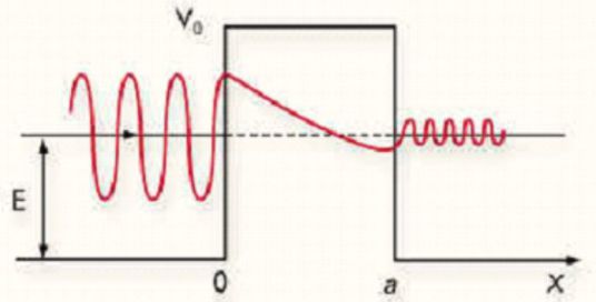
Give, without any prior calculation, the shape of the density of probability of the electron in function of \(x\).
Solution
Numeric value :
\(\alpha \approx {10^{10}}{m^{ - 1}}\;;\;\alpha L \approx 10\;so\;{e^{\alpha L}} > > {e^{ - \alpha L}}\)
Then :
\(t = \frac{F}{A} \approx \frac{4}{{\left( {1 + \frac{{i\alpha }}{k}} \right)\left( {1 - \frac{{ik}}{\alpha }} \right){e^{\alpha L}}{e^{ikL}}}} = \frac{{4{e^{ - \alpha L}}}}{{2 + \frac{{i\alpha }}{k} - \frac{{ik}}{\alpha }}}{e^{ - ikL}}\)
The transmission factor \(T\) of the potential barrier is :
\(T = \frac{{\left| {{J_t}} \right|}}{{\left| {{J_i}} \right|}} = \frac{{\left( {p_t^2/2m} \right){{\left| F \right|}^2}}}{{\left( {p_i^2/2m} \right){{\left| A \right|}^2}}} = {\left| {\frac{{4{e^{ - \alpha L}}}}{{2 + \frac{{i\alpha }}{k} - \frac{{ik}}{\alpha }}}} \right|^2}\)
Hence :
\(T = \frac{{16{k^2}{\alpha ^2}}}{{{{({\alpha ^2} + {k^2})}^2}}}{e^{ - 2\alpha L}} = \frac{{16E({U_0} - E)}}{{U_0^2}}\exp \left( { - 2\alpha L} \right)\)
Question
Compute the relative variation of the current of a quantum tunneling microscope when the space between the tip and the sample changes of \(0,1\) \(nm\). Comment this result.
Solution
The ratio of the two respective transmission coefficients \(T_1\) and \(T_2\) for the distances \(L_1=1\) \(nm\) and \(L_2=1,1\) \(nm\) is :
\(\frac{{{T_1}}}{{{T_2}}} = \exp (2\alpha ({L_2} - {L_1})) \approx {e^2} \approx 7\)
The electric current is divided by almost \(10\).
The atoms which had the dimension of a few nanometers can now be revealed by the variations of electric current during the sweeping of the surface of the sample by the sensor.
Question
In reality, the potential is not constant in empty space and changes of \(\Delta U_0=2\) \(eV\) between \(x=0\) and \(x=L\) (see figure above).
How can the evolution of transmission coefficient of the probability current \(T\) be anticipated ?
How can the new value of the relative variation of current calculated in the previous question be evaluated ?
Solution
One simple idea is to chose \(U_0=5\) \(eV\), the average value for \(U_0\).
Then \(\alpha\) diminishes of approximately \(0,9\) and \(T_1/T_2\) is approximately equal to \(6\).
The transmission of the barrier can also be calculated, by noticing that :
\(\frac{{dT}}{T} = - 2\alpha dL\)
Then :
\(\ln T = - 2\int_0^L {\sqrt {\frac{{2m(U(x) - E)}}{{{\hbar ^2}}}} dL = } - 2\int_0^L {\frac{{\sqrt {2m({U_0} - \Delta {U_0}(x/L) - E)} }}{\hbar }dL}\)