Quantum mechanics

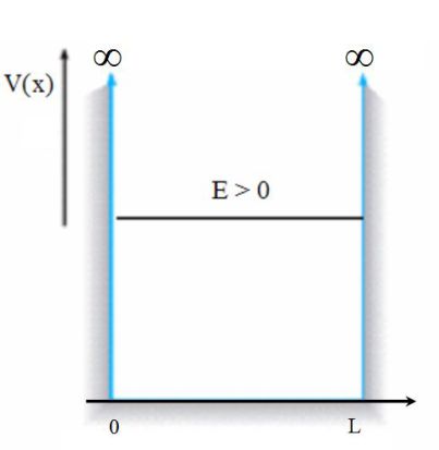
The case studied is a particle of mass \(m\) under the effect of a potential well.

An electron around a nucleus, free electrons in a metal (constant potential with a potential barrier at the border of the sample), or even a nucleon in the nucleus (strong interaction) are relevant examples.

In this lesson, the simple case of an infinite potential well in one dimension is considered.

Other more complicated cases will be studied in the exercises.

The potential in the well is considered constant and equal to zero. In quantum mechanics, the potential energy and the potential are two identical notions.

Let \(L\) be the width of the well.

We wish to determine the function of stationary states in the well, and then prove that the energy of the particle is quantified.

Let us resolve Schrödinger's stationary equation.

Inside the well, when the potential is equal to zero, this equation is :

\(- \frac{{{\hbar ^2}}}{{2m}}\frac{{{d^2}\varphi (x)}}{{d{x^2}}} = E\varphi (x)\)

Hence :

\(\frac{{{d^2}\varphi (x)}}{{d{x^2}}} + \frac{{2mE}}{{{\hbar ^2}}}\varphi (x) = 0\)

The energy is only kinetic, and it can be expressed as :

\(E=\frac {p^2}{2m}\)

Thus, it is positive and the solutions of Schrödinger's equation are of the following kind :

\(\varphi (x) = A\cos (kx) + B\sin (kx)\;\;\;(k = \sqrt {\frac{{2mE}}{{{\hbar ^2}}}})\)

The wave function is nil at the borders of the well (the continuity of the wave function is applied here in \(x=0\) and \(x=L\)).

Hence :

\(\varphi (0) = 0 = A\;\;\;\;\;\;\;so\;\;\;\;\;\;\;A = 0\)

And :

\(\varphi (L) = 0 = B\sin (kL)\;\;\;\;\;\;\;so\;\;\;\;\;\;\;\sin (kL) = 0\)

The last equation allows us to write :

\(kL=n\pi\)

\(n\) is an integer.

The wave vector is equal to :

\(k=\frac {2\pi}{\lambda}\)

Hence the equation :

\(L=n\frac {\lambda}{2}\)

The conditions of existence of stationary waves on a string and on acoustic tubes can be recognized here.

The states found are stationary.

The half­wavelength is a multiple of the width of the well.

The energy of the particle is hence quantified.

It can indeed be written :

\(E=\frac {p^2}{2m}=\frac {\hbar^2 k^2}{2m}\)

With :

\(k=\frac {2\pi}{\lambda}=\frac {n\pi}{L}\)

Then :

\({E_n} = {n^2}\frac{{{\hbar ^2}{\pi ^2}}}{{2m{L^2}}}\;\;\;\;\; ;\;\;\;\;\;{E_n} = {n^2}{E_1}\;\;\;\;\; ;\;\;\;\;\;{E_1} = \frac{{{\hbar ^2}{\pi ^2}}}{{2m{L^2}}}\)

The containment of the quanta particle in the infinite potential well induces the quantification of its energy.

This energy can only be an multiple integer of the energy \(E_1\) in the fundamental state of the particle.

The expression of the stationary wave function is :

\({\varphi _n}(x) = \sqrt {\frac{2}{L}} \sin \left( {\frac{{n\pi x}}{L}} \right)\;\;\;\;\;\;\;\;\;\;with\;\;\;\;\;\;\;\;\;\;\int_0^L {{{\left| {{\varphi _n}(x)} \right|}^2}dx} = 1\)

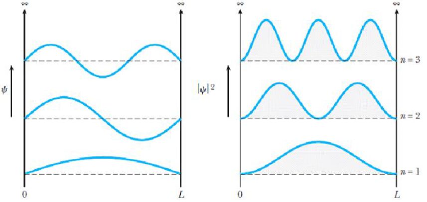
The previous figures illustrate the wave function and the density of probability (square of wave function) for the fundamental state (\(n=1\)) and two excited levels \(n=2\) and \(n=3\).

The notions of nodes and antinodes introduced in the study of stationary waves in a string or acoustic tube can be recognized.