Electromagnetic waves in plasmas
Fondamental : Definition of a plasma
Matter as we know it on Earth can exist mainly in three forms very familiar forms : solid, liquid and gas.
But there is a fourth state of matter, called plasma, obtained when the material is carried, for example at very high temperatures.
Paradoxically, it is this state that is on the scale of the Universe, the most common since astrophysicists estimate that \(99\)% of the material is in the plasma state in the Universe.
A plasma is a medium composed of atoms or molecules partially or completely ionized but remains electrically neutral overall ; thus, a hydrogen plasma is composed of hydrogen atoms, protons (hydrogen nuclei) and free electrons in various proportions depending on the nature of the plasma (little dense plasma or otherwise completely ionized).
The charged particles (ions and electrons) constituting the plasma interact through electromagnetic forces.
The existence of long-range forces allows a particle to interact with many others, giving a collective nature of these interactions.
This collective nature was particularly shown by longitudinal oscillations, studied in 1925 by Irving Langmuir. A certain amount of electrons moved from its equilibrium position, leaves the loss of charge becomes a charge of positive space ; this results in a restoring force due to the electric field which tends to return the electrons to their equilibrium position.
The creation of a plasma requires a significant energy input.
This can be done by heating, by bombardment with a very intense laser beam or by electric discharge in a gas subjected to a very high potential difference (in devices known as gas discharge tubes).
Traditionally, there are two kinds of plasmas : the "cold" plasmas whose temperature remains below \(\approx 10^5\;K\) and "hot" plasmas whose temperatures exceed \(\approx 10^6\;K\).
Examples of plasmas in nature are numerous ; we can cite :
Magnetosphere and ionosphere.
The heart of stars, eg hot and dense plasmas.
Neon tubes and the phenomenon of lightning (electrical shock).
The applications of plasma physics are very diverse and growing in fields as varied as :
Thermonuclear fusion : by producing a plasma of very high density and very high temperatures, physicists hope to initiate nuclear fusion reactions and create a considerable energy generator.
Electronics : the use of cold plasmas allows the integration of electronic circuits. Television has a plasma screen.
Materials processing : plasmas used to destroy, transform, analyze, weld, create ... matter. For example, plastic fibers may be treated by plasma to become waterproof.
If the energy input is considerable, the atoms nuclei can be separated into their prime constituents, the nucleons (protons and neutrons) : the plasma obtained is then a mixture of nucleons and electrons.
At higher energy again (when such collisions performed at almost equal speed of light between atomic nuclei), the nucleons can disintegrate into their ultimate constituents, the quarks and gluons (particles responsible for the cohesion of quarks in atomic nuclei). The "soup" thus obtained is called quark-gluon plasma. According to the theory of "Big Bang", such a quark-gluon plasma could have existed in the first microseconds of existence of the Universe.
Complément : Some videos on plasmas
Fondamental : Plasma model
In the following, we choose a plasma model consisting \(n\) ions (mass \(M\) and load \(+e\)) and \(n\) electrons (mass \(m\) and load \(-e\)) per unit volume.
Neglecting all interactions between ions, neither attraction or electrostatic repulsion nor collision. This assumption is satisfied for a little dense plasma.
The ionosphere is the part of the upper atmosphere (\(75-250 \; km\) altitude in several layers) where the gases are ionized by cosmic radiation and the solar wind : this is an example of such plasma.
Note \(\vec V\) and \(\vec v\) mesoscopic velocity of an ion and an electron.
If an external electric field is applied to plasma :
\(M\frac{{d\vec V}}{{dt}} = e\vec E\;\;\;\;\;\;\;\;and\;\;\;\;\;\;\;m\frac{{d\vec v}}{{dt}} = - e\vec E\)
Therefore :
\(\frac{{d\vec V}}{{dt}} = - \frac{m}{M}\frac{{d\vec v}}{{dt}}\)
Or, to a constant :
\(\vec V = - \frac{m}{M}\vec v\)
Therefore, with \(m/M<<1\), the speed of the positive ions is very low with respect to that of electrons.
We only take into account the movement of electrons.
The volume density of the plasma :
\(\vec j = - ne\vec v + ne\vec V = - ne\left( {1 + \frac{m}{M}} \right)\;\vec v \approx - ne\vec v\)
It is substantially equal to that of the electrons.
Fondamental : Maxwell equations in the plasma
We are interested in the propagation of a monochromatic progressive plane electromagnetic wave in a plasma.
One notes \(\vec E\) and \(\vec B\) the electric and magnetic fields associated with this wave.
These fields act on the plasma electrons and start moving.
The equation of motion of an electron is :
\(m\frac{{d\vec v}}{{dt}} = - e\;\vec E - e\;\vec v \wedge \vec B\)
Assuming (as a wave in vacuum), \(B/E \approx 1/c\), we see that as long as the ions are not relativist :
\(\left\| {e\;\vec v \wedge \vec B} \right\| < < eE\)
This will neglect the magnetic force with respect to the electric force to study the motion of electrons :
\(m\frac{{d\vec v}}{{dt}} = - e\;\vec E\)
Maxwell's equations are written, noting that the volume charge density is zero (plasma remains neutral overall) :
\(\left\{ \begin{array}{l}div\;\vec E = 0 \\div\;\vec B = 0 \\\overrightarrow {rot} \;\vec E = - \frac{{\partial \vec B}}{{\partial t}} \\\overrightarrow {rot} \;\vec B = {\mu _0}\vec j + {\varepsilon _0}{\mu _0}\frac{{\partial \vec E}}{{\partial t}} \\\end{array} \right.\)
With :
\(\frac{{\partial \vec j}}{{\partial t}} = - ne\frac{{\partial \vec v}}{{\partial t}} = \frac{{n{e^2}}}{m}\vec E\)
Fondamental : Propagation equation and dispersion relation of monochromatic traveling plane electromagnetic waves
Relationship of the vector analysis is used to decouple the Maxwell equations and obtain the propagation equation verified by the electric field \(\vec E\) :
\(\overrightarrow {rot}( \overrightarrow {rot} \vec E) = \overrightarrow {grad} (div\vec E) - \Delta \vec E\)
So :
\(\overrightarrow {rot} (\overrightarrow {rot} \vec E) = - \frac{\partial }{{\partial t}}(\overrightarrow {rot} \vec B) = - \frac{\partial }{{\partial t}}\left( {{\mu _0}\vec j + {\varepsilon _0}{\mu _0}\frac{{\partial \vec E}}{{\partial t}}} \right) = - {\mu _0}\frac{{n{e^2}}}{m}\vec E - {\varepsilon _0}{\mu _0}\frac{{{\partial ^2}\vec E}}{{\partial {t^2}}} = - \Delta \vec E\)
We obtain :
\({\mu _0}\frac{{n{e^2}}}{m}\vec E + \frac{1}{{{c^2}}}\frac{{{\partial ^2}\vec E}}{{\partial {t^2}}} = \Delta \vec E\)
It is the propagation equation satisfied by the electric field \(\vec E\).
We seek a complex harmonic solution of the wave equation in the form :
\(\underline {\vec E} = {\underline {\vec E} _0}{e^{i(\omega t - \vec k.\vec r)}}\;\;\;\;\;\;\;\;\;and\;\;\;\;\;\;\;\;\;\;\underline {\vec B} = {\underline {\vec B} _0}{e^{i(\omega t - \vec k.\vec r)}}\)
It comes :
\(\frac{{{\partial ^2}\vec E}}{{\partial {t^2}}} = - {\omega ^2}\vec E\;\;and\;\;\Delta \vec E = - {\underline k ^2}\vec E\)
Hence :
\({\underline k ^2} = \frac{{{\omega ^2} - \omega _p^2}}{{{c^2}}}\)
With :
\(\omega _p^2 = \frac{{{\mu _0}{c^2}n{e^2}}}{m}\) (\(\omega_p\) is called plasma frequency)
This is the Klein-Gordon dispersion relation.
Two cases are considered :
If \(\omega < \omega_p\), then \(\underline k\) is pure imaginary :
\(\underline k = \pm i\sqrt {\frac{{\omega _p^2 - {\omega ^2}}}{{{c^2}}}} = \pm i{k_2}\)
The electric field of the wave is then written in the form :
\(\underline {\vec E} = {\underline {\vec E} _0}{e^{i(\omega t)}}{e^{ \pm {k_2}x}}\;\;\;\;\;\;\;\;\;\;so\;\;\;\;\;\;\;\;\;\;\vec E = {\vec E_0}{e^{ \pm {k_2}x}}\cos (\omega t + {\phi _0})\)
This gives a standing wave so-called evanescent (exponential changes in amplitude in the direction of the wave).
If \(\omega > \omega_p\), \(k\) is real and equal to :
\(k = \pm \sqrt {\frac{{{\omega ^2} - \omega _p^2}}{{{c^2}}}}\)
There is propagation without absorption.
The plasma acts as a high-pass filter with cut-off frequency \(\omega_p\).
Fondamental : Phase velocity and group velocity
It is in the case where there is a propagation (hence, \(\omega > \omega_p\)) :
The wave propagates in the direction of \(x>0\) is :
\(k = \sqrt {\frac{{{\omega ^2} - \omega _p^2}}{{{c^2}}}}\)
The relationship between \(k\) and \(\omega\) is nonlinear : the medium is dispersive.
For a real wave, which is the superposition of monochromatic progressive plane waves propagating in any medium, it is possible to define two speeds : the phase velocity and the group velocity.
The phase velocity is :
\({v_\varphi }(\omega ) = \frac{\omega }{k} = \frac{1}{{\sqrt {1 - \frac{{\omega _p^2}}{{{\omega ^2}}}} }}\;c\)
We note that \(v_{\varphi}>c\) ; this is not paradoxical because this speed does not match the speed of information or energy (in the case of the group velocity).
The group velocity is defined as :
\({v_g} = \frac{{d\omega }}{{dk}}\)
This is the propagation velocity of the envelope of the wave (see the lecture note on the group velocity).
It shows that it is usually identified with the speed of propagation of energy (or information).
The principle of relativity requires that the group velocity is less than the speed of light in vacuum.
To calculate, we can differentiate the dispersion relation written in the form :
\({k ^2} = \frac{{{\omega ^2} - \omega _p^2}}{{{c^2}}}\)
So :
\(2kdk=\frac {1}{c^2}2\omega d\omega\)
We obtain :
\(v_{\varphi}v_g=c^2\)
And, finally :
\({v_g} = \sqrt {1 - \frac{{\omega _p^2}}{{{\omega ^2}}}} \;\;c\)
Note that \(v_g<c\).
A real physical wave, consisting of sinusoidal progressive plane waves, will deform during its propagation : this is called dispersion.
Fondamental : Structure of the harmonic progressive plane wave
Maxwell's equations :
\(div \vec E =0\), \(div \vec B =0\) and \(\overrightarrow {rot} \;\vec E = - \frac{{\partial \vec B}}{{\partial t}}\)
Give, in complex notation :
\(\vec k.\underline {\vec E} = \vec k.\underline {\vec B} = 0\;\;\;\;\;\;\;\;\;\;and\;\;\;\;\;\;\;\;\;\;\vec k \wedge \underline {\vec E} = \omega \underline {\vec B}\)
In real notation :
\(\vec k.\vec E = \vec k.\vec B = 0\;\;\;\;\;\;\;\;\;\;and\;\;\;\;\;\;\;\;\;\vec B = \frac{{\vec k \wedge \vec E}}{\omega }\;\)
The triad \((\vec E,\vec B,\vec k)\) is direct and :
\(B = \;\frac{{kE}}{\omega } = \frac{E}{{{v_\varphi }}}\)
The structure of the monochromatic progressive plane wave is similar to that of vacuum (only the phase velocity is different and depends on the wave frequency).
Exemple : Some orders of magnitude
The ionosphere is the part of the upper atmosphere ( altitude of \(75-250 \;km\) in several layers) where the gases are ionized by cosmic radiations and the solar wind.
The particle density of electrons in the ionosphere is from about \(10^{10}\;m^{-3}\) to \(10^{12}\;m^{-3}\) and the plasma frequency about \(\nu_p=10^7\;Hz\).
For \(\nu=10^5\;Hz<\nu_p\), the ionosphere acts as a reflector : this explains the first transatlantic radio connection made by Marconi in 1901.
Thus, amplitude modulation radio waves can reach distant points on the globe.
For \(\nu=10^8\;Hz>\nu_p\), the ionosphere is "transparent". These frequencies are used to communicate with satellites.
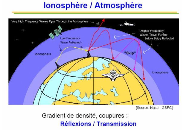
Reference : NASA
Another example : France inter GO et France Info FM
The frequency of France Inter GO is \(f_{GO}=164\;kHz\) and the frequency of France Info FM is \(f_{FM}=105,5\;MHz\).
We see that \(f_{GO}<\nu_p<f_{FM}\) : GO reflect off the ionosphere and can be received at much greater distances from the place of issue than France Info whose waves propagate in the ionosphere.
Complément : To go further ...
"Propagation of radio wave through the atmosphere" :
Propagation through the troposphere
Propagation through the ionosphere
By Laurent Castanet and Patrick Lassudrie-Duchesne.