Electromagnetic energy review
Fondamental : Density of power given by the electromagnetic field to matter
An electromagnetic field will interact with charged particles and give them energy.
In fact, a charge \(q\) is subject to Lorentz' force from this electromagnetic field, which has a power of :
\(P_L = q(\vec E + \vec v \wedge \vec B).\vec v = q\;\vec E.\vec v\)
By writing \(n\) the number of charge carriers by volume unit, the density of power given by the electromagnetic field to matter is expressed by :
\(p_L = \frac{{dP_L }}{{d\tau }} = nq\;\vec E.\vec v = \vec j.\vec E\)
Remark :
The power received by the electromagnetic field from charge carriers is equal to \(-p_L\) (do the analogy with \(p_S\), the density of power received by a heat-conductor setting from the heat sources, see below).
Rappel : Energy conservation equation in conductive phenomena (see lesson about thermal transfers)
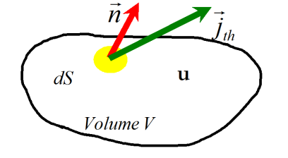
Let us consider a volume \((V)\) delimited by a closed surface \((S)\) (steady in the referential of study).
The total internal energy \(U(t)\) included in the volume at the time t is :
\(U(t) = \iiint_{(V)} u(M,t)\;d\tau\)
Where \(u(M,t)\) is the density of internal energy.
The internal energy conservation allows us to write :
\(\frac{{dU}}{{dt}} = -\oint_{(S)}\vec {j}_{th}.\vec{n} \ dS + \iiint_{(V)} p_s (M,t)\;d\tau\)
The volume \((V)\) is steady, so :
\(\frac{{dU}}{{dt}} = \frac{d}{{dt}}\left( { \iiint_{(V)} u\;d\tau} \right) =\iiint_{(V)} \frac{\partial u(M,t)}{\partial t}d\tau\)
By using the divergence theorem (or Green - Ostrogradsky's law), it comes :
\(\iiint_{(V)} \frac{\partial u(M,t)}{\partial t}d\tau= \iiint_{(V)} \left( {( - div\vec j_{th} \; + p_s (M,t))d\tau } \right)\)
This result is true for any volume \((V)\), so :
\(\frac{{\partial u(M,t)}}{{\partial t}} = - div\vec j_{th} + p_s (M,t)\)
This equation had been proven in the one dimension case.
Fondamental : Local conservation of electromagnetic energy equation
By using the analogy with conservation equations (charge, mass, diffusion, heat) we would like to get an equation of this kind :
\(\frac{{\partial e_{em} }}{{\partial t}} = - div\;\vec \Pi + ( - \vec j.\vec E)\)
Where \(e_{em}\) represents the density of electromagnetic energy (included in the electromagnetic field).
\( \vec \Pi\) is a vector called the "Poynting vector".
It is supposed to give the direction of the electromagnetic energy exchanges (especially by calculating its flux through a surface).
The following calculation is not on the curriculum :
The product \(\vec j .\vec E\) can be expressed as such by using Maxwell - Ampere's equation :
\(\overrightarrow {rot} \;\vec B = \mu _0 \vec j + \varepsilon _0 \mu _0 \frac{{\partial \vec E}}{{\partial t}}\)
\(\vec j.\vec E = \frac{1}{{\mu _0 }}\vec E.\overrightarrow {rot} \;\vec B - \varepsilon _0 \vec E.\frac{{\partial \vec E}}{{\partial t}} = \frac{1}{{\mu _0 }}\vec E.\overrightarrow {rot} \;\vec B - \frac{1}{2}\varepsilon _0 \frac{{\partial (\vec E^2 )}}{{\partial t}}\)
By writing that :
\(div(\vec E \wedge \vec B) = \vec B.\overrightarrow {rot} \;\vec E - \vec E.\overrightarrow {rot} \;\vec B = \vec B.\left( { - \frac{{\partial \vec B}}{{\partial t}}} \right) - \vec E.\overrightarrow {rot} \;\vec B\)
Hence :
\(\vec E.\overrightarrow {rot} \;\vec B = - \frac{1}{2}\frac{{\partial (\vec B^2 )}}{{\partial t}} - div(\vec E \wedge \vec B)\)
Thus :
\(\vec j.\vec E = - \frac{1}{{2\mu _0 }}\frac{{\partial (\vec B^2 )}}{{\partial t}} - \frac{1}{{\mu _0 }}div(\vec E \wedge \vec B) - \frac{1}{2}\varepsilon _0 \frac{{\partial (\vec E^2 )}}{{\partial t}}\)
Then :
\(\frac{\partial }{{\partial t}}\left[ {\frac{{\varepsilon _0 \vec E^2 }}{2} + \frac{{\vec B^2 }}{{2\mu _0 }}} \right] = - div(\frac{{\vec E \wedge \vec B}}{{\mu _0 }}) + ( - \vec j.\vec E)\)
Can be written :
Electromagnetic density of energy :
\(e_{em} = \frac{{\varepsilon _0 \vec E^2 }}{2} + \frac{{\vec B^2 }}{{2\mu _0 }}\)
Poynting vector :
\(\vec \Pi = \frac{{\vec E \wedge \vec B}}{{\mu _0 }}\)
Thus the equation can be written this way :
\(\frac{{\partial e_{em} }}{{\partial t}} = - div\;\vec \Pi +(- \vec j.\vec E)\)
And thus corresponds to an electromagnetic energy assessment.
Attention : Poynting Energy assessment
Density of electromagnetic energy :
\(e_{em} = \frac{{\varepsilon _0 \vec E^2 }}{2} + \frac{{\vec B^2 }}{{2\mu _0 }}\)
Poynting vector :
\(\vec \Pi = \frac{{\vec E \wedge \vec B}}{{\mu _0 }}\)
Local conservation of electromagnetic energy :
\(\frac{{\partial e_{em} }}{{\partial t}} = - div\;\vec \Pi+( - \vec j.\vec E)\)
The integral form of the conservation of electromagnetic energy is :
\(\frac{d}{dt}(\iiint_V e_md\tau)=- \oint_S\vec {\vec \Pi}.\vec{n} \ dS +\iiint_V (-\vec j .\vec E) d\tau\)
Remarque : Energy propagation velocity
By proceeding to an analogy with the charge conservation equation, an energy propagation speed (written \(\vec u\)) can be defined with this relation :
\(\vec u = \frac{{\vec \Pi }}{{e_{em} }}\) (analogy : \(\vec v=\vec j /\rho_{mobile}\)
Exemple : Energy balance for the conductive energetic field
Let us consider a conductive thread of conductivity \(\gamma\), associated to a cylinder of axis \((Oz)\) and of radius \(a\).
A steady and uniform electric field reigns, both inside and outside the wire :
\(\vec E = E_0 \;\vec u_z\)
The wire is then crossed by volumic currents of uniform density :
\(\vec j = j \vec u_z = \gamma E_0 \vec u_z\)
The magnetic field created by this distribution is of this kind :
\(\vec B=B(r)\vec u_{\theta}\)
It can be computed using Ampere's circuital law.
By writing \(I=\pi a^2\) the total current crossing the transversal section of the wire, then :
If \(r<a\) :
\(\vec B(r) = \frac{{\mu _0 I}}{{2\pi \;a^2 }}\;r\;\vec u_\theta\)
If \(r>a\) :
\(\vec B(r) = \frac{{\mu _0 I}}{{2\pi }}\frac{1}{r}\;\vec u_\theta\)
Poynting's vector is :
\(\vec \Pi = \frac{{\vec E \wedge \vec B}}{{\mu _0 }}\)
Thus :
If \(r<a\) :
\(\vec \Pi = - \frac{{E_0 I}}{{2\pi \;a^2 }}\;r\;\vec u_r\)
If \(r>a\) :
\(\vec \Pi = - \frac{{E_0 I}}{{2\pi }}\frac{1}{r}\;\vec u_r\)
The general expression of electromagnetic energy conservation is reminded :
\(\iiint_{(V)} \frac{\partial e_{em}}{\partial t}d\tau=- \oint_{(S)}\vec {\vec \Pi}.\vec{n} \ dS - \iiint_{(V)} \vec j .\vec E d\tau\)
In the particular case of steady-state :
\(\oint_{(S)}\vec {\vec \Pi}.\vec{n} \ dS=-\iiint_{(V)} \vec j .\vec E d\tau=-\iiint_{(V)} \frac{j^2}{\gamma}d\tau\)
Physically, in steady-state, the power dissipated by Joule effect is evacuated outside the volume \((V)\).
We compute the exiting flux of the Poynting vector through a cylinder of \(Oz\) axis and radius \(r\).
If \(r<a\) :
\(\Phi = - \frac{{E_0 I}}{{\pi a^2 }}\pi r^2 h = - \frac{{j^2 }}{\gamma }\pi r^2 h\)
If \(r>a\) :
\(\Phi = - \frac{{E_0 I}}{{\pi a^2 }}\pi a^2 h = - \frac{{j^2 }}{\gamma }\pi a^2 h\)
We can recognize easily, in both cases, the power absorbed by Joule effect in the cylinder of radius \(r\) considered (the volumic Joule dissipated power is \(p_J=\vec j \vec E = j^2 /\gamma\)).
The previous conservation equation is verified.