Linear filtering
Fondamental :
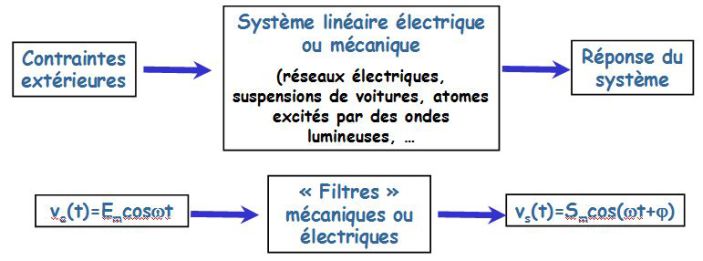
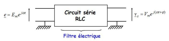
Harmonic analysis (or frequential) of a system is its study through its harmonic response \(s(t)\), that is to say, its response in sinusoidal permanent regime when subjected to a sinusoidal input \(e(t)\) which is varied frequency \(\omega\).
Filter \(1st\) order :
Example of a low-pass filter :
\({\underline v _s}(t) = \underline H (j\omega ){\underline v _e}(t) = \frac{K}{{1 + j\omega \tau}}{\underline v _e}(t)\)
Example of a high-pass filter :
\({\underline v _s}(t) = \underline H (j\omega ){\underline v _e}(t) = K\frac{j\omega \tau}{{1 + j\omega \tau}}{\underline v _e}(t)\)
\(\tau=1/\omega_c\), with \(\omega_c\) the cut-off frequency to \(-3\;dB\).
Filter \(2nd\) order :
Example of a low-pass filter :
\({\underline v _s}(t) = \underline H (j\omega ){\underline v _e}(t) = \frac{K}{{1 - \frac{{{\omega ^2}}}{{\omega _0^2}} + 2j\sigma \frac{\omega }{{{\omega _0}}}}}{\underline v _e}(t)\)
where \(\omega_0\) is the natural angular frequency of the filter and \(\sigma\) the damping coefficient.
\(Q=1/2\sigma\) is defined as the quality factor.
Example of a high-pass filter :
\({\underline v _s}(t) = \underline H (j\omega ){\underline v _e}(t) = K\frac{\frac{{{\omega ^2}}}{{\omega _0^2}} }{{1 - \frac{{{\omega ^2}}}{{\omega _0^2}} + 2j\sigma \frac{\omega }{{{\omega _0}}}}}{\underline v _e}(t)\)
Example of a bandpass filter :
\({\underline v _s}(t) = \underline H (j\omega ){\underline v _e}(t) = K\frac{2j\sigma\frac{\omega}{\omega_0} }{{1 - \frac{{{\omega ^2}}}{{\omega _0^2}} + 2j\sigma \frac{\omega }{{{\omega _0}}}}}{\underline v _e}(t)=\frac{K}{1+jQ(\frac{\omega}{\omega_0}-\frac{\omega_0}{\omega})}\underline v_e(t)\)
\(\omega_0\) here is also the band-pass filter resonance pulse.
Example of a notch filter (or band-stop) :
\({\underline v _s}(t) = \underline H (j\omega ){\underline v _e}(t) = K\frac{1-\frac{{{\omega ^2}}}{{\omega _0^2}} }{{1 - \frac{{{\omega ^2}}}{{\omega _0^2}} + 2j\sigma \frac{\omega }{{{\omega _0}}}}}{\underline v _e}(t)\)
Définition : General notations and definitions
We note : (in complex notations)
\({\underline v _e}(t) = {V_{em}}{e^{j\omega t}}\;\;\;\;\;;\;\;\;\;\;\;{\underline v _s}(t) = {V_{sm}}{e^{j\varphi }}{e^{j\omega t}}\)
\(\varphi\) is the phase shift of the output voltage with respect to the filter input voltage.
\(\underline H(j\omega)\) is the voltage transfer function of the filter :
\(\underline H (j\omega ) = \frac{{{{\underline v }_s}}}{{{{\underline v }_e}}} = \frac{{{V_{sm}}}}{{{V_{em}}}}{e^{j\varphi }}\)
And :
\(G(\omega)\) is the real gain :
\(G(\omega ) = \left| {\underline H (j\omega )} \right| = \frac{{{V_{sm}}}}{{{V_{em}}}}\)
\(G_{dB}\) is the gain in decibels (\(dB)\) :
\({G_{dB}}(\omega ) = 20\log G(\omega ) = 20\log \left( {\frac{{{V_{sm}}}}{{{V_{em}}}}} \right)\)
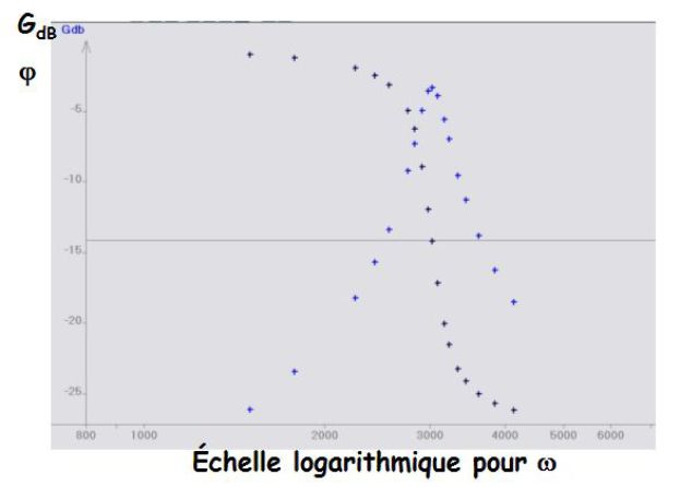
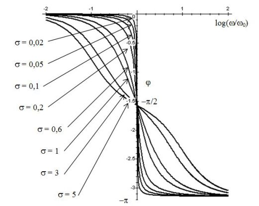
The previous figure gives a Bode diagram of a band-pass filter, that is to say, the graphical representation of the gain in \(dB\) (\(G_{dB}(\omega)\)) and the phase shift \(\varphi(\omega)\) as a function of the pulse \(\omega\) and on a logarithmic scale.
Fondamental : Fundamental filtering 1st order (eg RC series circuit)
Studying an RC series circuit and measuring the output voltage \(\underline v_s\) in the open output.
Qualitative study of the nature of flitre :
At low frequencies, the capacitor is equivalent to an open switch (its impedance \(1/C\omega\) is infinite).
The current in the circuit is zero. Thus, the voltage at the \(R\) terminal is also zero and therefore \(\underline v_s=\underline v_e\).
At high frequency, the capacitor is equivalent to a zero resistance wire. So, \(\underline v_s=0\).
The filter studied here is thus a low-pass filter.
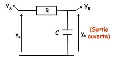
Open output, the voltage divider rule gives :
\({\underline v _s} = \frac{{\frac{1}{{jC\omega }}}}{{R + \frac{1}{{jC\omega }}}}{\underline v _e}\;\;\;\;\;so\;\;\;\;\;\underline H (j\omega ) = \frac{{{{\underline v }_s}}}{{{{\underline v }_e}}} = \frac{1}{{1 + jRC\omega }} = \frac{1}{{1 + j\frac{\omega }{{{\omega _0}}}}}\)
With :
\(\omega_0=\frac{1}{RC}\)
The natural angular frequency of the filter, which is also the cut-off frequency to \(-3\;dB\), that is to say the pulse for which the real gain is \(G_{max}/\sqrt{2}\),or, what is equivalent, \(G_{dB}(\omega_0)=G_{dB,max}-3\;dB\).
It is the transfer function of a low-pass filter of the first order.
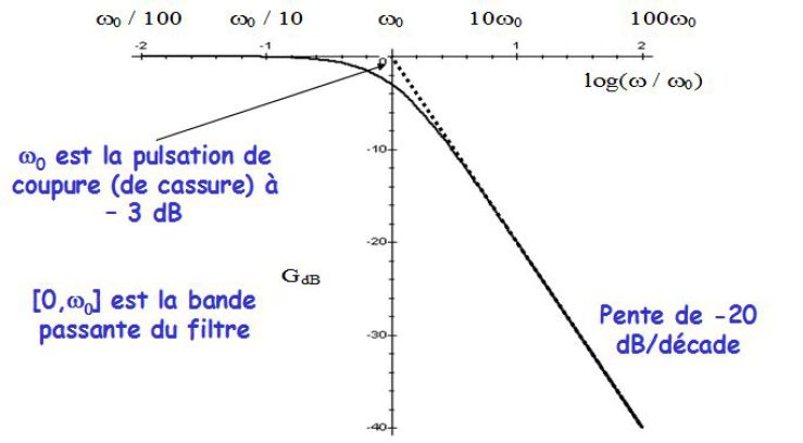
The figure above shows the Bode amplitude of this low-pass filter of the first order.
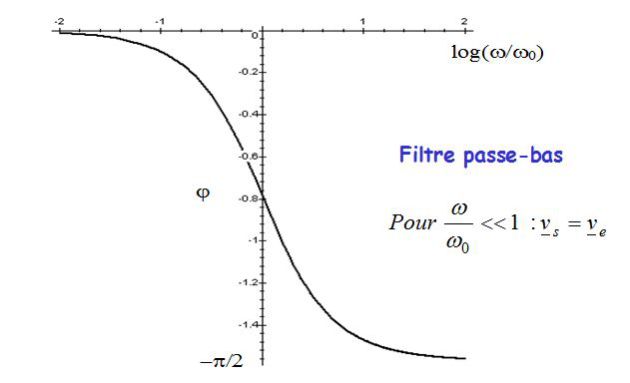
The following figure shows the Bode phase.
Other filter \(1st\) order :
RC series, output voltage across \(R\) :
It is a high-pass filter.
\(\underline H (j\omega ) = \frac{{{{\underline v }_s}}}{{{{\underline v }_e}}} = \frac{{j\frac{\omega }{{{\omega _0}}}}}{{1 + j\frac{\omega }{{{\omega _0}}}}} = \frac{1}{{1 - j\frac{{{\omega _0}}}{\omega }}}\)
With \(\omega_0=1/RC\).
Circuit RL series, output voltage across \(L\) :
It is a high-pass filter.
\(\underline H (j\omega ) = \frac{{{{\underline v }_s}}}{{{{\underline v }_e}}} = \frac{{j\frac{\omega }{{{\omega _0}}}}}{{1 + j\frac{\omega }{{{\omega _0}}}}} = \frac{1}{{1 - j\frac{{{\omega _0}}}{\omega }}}\)
With :
\(\omega_0=\frac{R}{L}\)
Circuit RL series, output voltage across \(R\) :
It is a low-pass filter.
\(\underline H (j\omega ) = \frac{{{{\underline v }_s}}}{{{{\underline v }_e}}} = \frac{1}{{1 + j\frac{\omega }{{{\omega _0}}}}}\)
With :
\(\omega_0=\frac{R}{L}\)
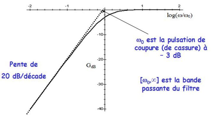

The preceding figures show the Bode diagram in amplitude and phase of a high-pass filter of the first order.
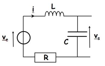
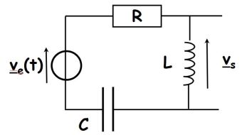
Fondamental : Filter 2nd order (eg the series RLC circuit)
It is a series RLC circuit as a quadrupole (Figure below).
The following table shows the nature of the filter obtained by the output dipole :
Dipole output | Filter obtained |
|
|
Fondamental : The terminals of C in open output : low - pass filter
The voltage divider rule gives :
\(\underline H (j\omega ) = \frac{{\frac{1}{{jC\omega }}}}{{R + jL\omega \; + \frac{1}{{jC\omega }}}} = \frac{1}{{1 - LC{\omega ^2} + jRC\omega \;}}\)
We want to write this transfer function in the standard form :
\(\underline H (j\omega ) = \frac{K}{{1 - \frac{{{\omega ^2}}}{{\omega _0^2}} + 2j\sigma \frac{\omega }{{{\omega _0}}}}}\)
For identification :
\(\omega _0^2 = \frac{1}{{LC}}\;\;\;\;\;;\;\;\;\;\;jRC\omega = 2j\sigma \frac{\omega }{{{\omega _0}}}\;\;\;\;\;;\;\;\;\;\;K = 1\)
Whence :
\({\omega _0} = \frac{1}{{\sqrt {LC} }}\;\;\;\;\;;\;\;\;\;\;\sigma = \frac{1}{2}RC{\omega _0} = \frac{R}{2}\sqrt {\frac{C}{L}} \;\;\;\;\;;\;\;\;\;\;K = 1\)
So :
\(\underline H (j\omega ) = \frac{1}{{1 - \frac{{{\omega ^2}}}{{\omega _0^2}} + 2j\sigma \frac{\omega }{{{\omega _0}}}}}\;\;\;\;\;\;\;so\;\;\;\;\;\;\;\;\left\{ \begin{array}{l}G(\omega ) = \frac{1}{{\sqrt {{{\left( {1 - \frac{{{\omega ^2}}}{{\omega _0^2}}} \right)}^2} + {{\left( {2\sigma \frac{\omega }{{{\omega _0}}}} \right)}^2}} }} \\\tan \varphi = - \frac{{2\sigma \frac{\omega }{{{\omega _0}}}}}{{1 - \frac{{{\omega ^2}}}{{\omega _0^2}}}}\;\;\;(\sin \varphi < 0,\;\varphi \in \left[ { - \pi ,0} \right]) \\\end{array} \right.\)
Referring to the study of mechanical oscillators (response in elongation), one obtains :
There are "resonance voltage" across \(C\) terminals ( "load resonance "), ie corresponding to a maximum voltage across \(C\), for the pulse of GBF \(\omega_r\) such that :
\(\;\omega _r^{} = \omega _0^{}\sqrt {1 - 2{\sigma ^2}} \;\;\;\;\;\;\;\left( {with\;\sigma < \frac{1}{{\sqrt 2 }}} \right)\)
And the maximum voltage across \(C\) at "load resonance" is :
\({V_{s,m}}({\omega _r}) = \frac{1}{{2\sigma \sqrt {1 - {\sigma ^2}} }}{V_{e,m}}\)
The above formulas become, using the quality factor \(Q\) in place of the damping coefficient \(\sigma\) (\(Q=1/2\sigma\)) :
\(\;\omega _r^{} = \omega _0^{}\sqrt {1 - \frac{1}{{2{Q^2}}}} \;\;\;\;\;\;\;\;\;\;with\;\;\;\;\;\;\;\;\;\;Q > \frac{1}{{\sqrt 2 }}\)
And :
\({V_{s,m}}({\omega _r}) = \frac{Q}{{\sqrt {1 - \frac{1}{{4{Q^2}}}} }}{V_{e,m}}\)
Note :
For low amortization (\(\sigma\) «small» and \(Q\) «large»), then :
\(\;\omega _r^{} \approx \omega _0^{}\;\;\;\;\;\;\;and\;\;\;\;\;\;\;{V_{s,m}}({\omega _r}) \approx Q{V_{e,m}}\)
Thus, if \(Q=10\), the amplitude at the resonance is \(10\) times that of the excitation : the resonance is termed "sharp" and may cause destruction of the oscillating system.
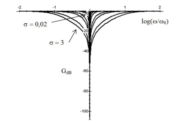
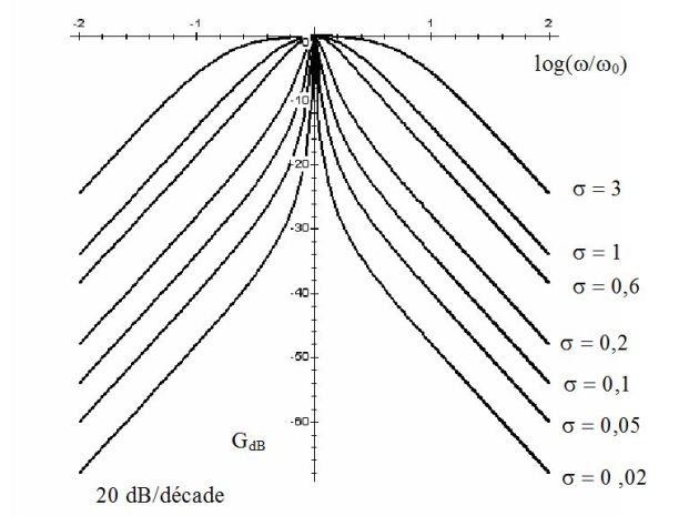
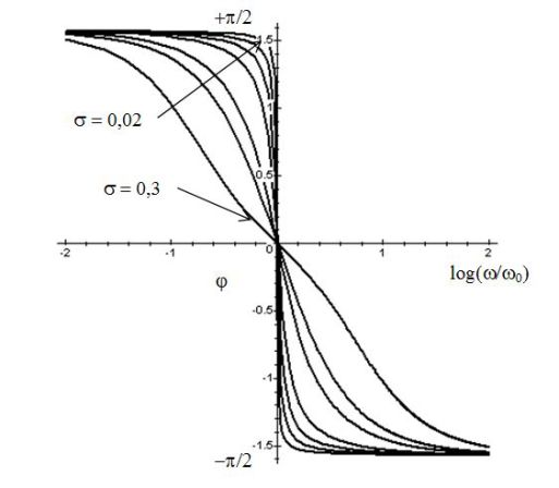
The following figures give the Bode diagram in gain and phase of a low-pass filter \(2nd\) order. Different numerical values of \(\sigma\) are used.

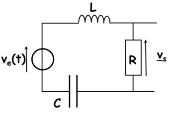
Fondamental : The terminals of R open output : band - pass filter
The voltage divider rule gives :
\(\underline H (j\omega ) = \frac{R}{{R + jL\omega \; + \frac{1}{{jC\omega }}}} = \frac{1}{{1 + \frac{j}{R}\left( {L\omega \; - \frac{1}{{C\omega }}} \right)\;}}\)
We want to write this transfer function in the standard form :
\(\underline H (j\omega ) = \frac{{2j\sigma \frac{\omega }{{{\omega _0}}}}}{{1 - \frac{{{\omega ^2}}}{{\omega _0^2}} + 2j\sigma \frac{\omega }{{{\omega _0}}}}}K = \frac{1}{{1 + \frac{j}{{2\sigma }}\left( {\frac{\omega }{{{\omega _0}}} - \frac{{{\omega _0}}}{\omega }} \right)}}K\)
For identification:
\(\frac{L}{R} = \frac{1}{{2\sigma {\omega _0}}}\;\;\;\;\;;\;\;\;\;\;\frac{1}{{RC}} = \frac{{{\omega _0}}}{{2\sigma }}\;\;\;\;\;;\;\;\;\;\;K = 1\)
Hence (Member to Member ratio) :
\(\omega _0^2 = \frac{1}{{LC}}\;\;\;\;\;;\;\;\;\;\;\sigma = \frac{R}{2}\sqrt {\frac{C}{L}} \;\;\;\;;\;\;\;\;\;K = 1\)
So :
\(\underline H (j\omega ) = \frac{{2j\sigma \frac{\omega }{{{\omega _0}}}}}{{1 - \frac{{{\omega ^2}}}{{\omega _0^2}} + 2j\sigma \frac{\omega }{{{\omega _0}}}}} = \frac{1}{{1 + \frac{j}{{2\sigma }}\left( {\frac{\omega }{{{\omega _0}}} - \frac{{{\omega _0}}}{\omega }} \right)}}\;\;\;\;\;\;\;so\;\;\;\;\;\;\;\left\{ \begin{array}{l}G(\omega ) = \frac{1}{{\sqrt {1 + \frac{1}{{4{\sigma ^2}}}{{\left( {\frac{\omega }{{{\omega _0}}} - \frac{{{\omega _0}}}{\omega }} \right)}^2}} }} \\\tan \varphi = - \frac{1}{{2\sigma }}\;\left( {\frac{\omega }{{{\omega _0}}} - \frac{{{\omega _0}}}{\omega }} \right)\;\;(\cos \varphi > 0,\;\varphi \in \left[ { - \frac{\pi }{2},\frac{\pi }{2}} \right]) \\\end{array} \right.\)
Resonant voltage across \(R\) ("resonance intensity") :
A go "resonance voltage" across \(R\) (« resonance current »), corresponding to a maximum voltage terminals \(R\), for a pulse GBF equal to the oscillation frequency \(\omega_0\) of the circuit (RLC) series :
\(\;{\omega _0} = \frac{1}{{\sqrt {LC} }}\)
And the maximum voltage across \(R\) for the "resonance current" is :
\({V_{s,m}} = {V_{e,m}}\)
The pass-band is :
\(\Delta \omega = {\omega _{{c_2}}} - {\omega _{{c_1}}} = \frac{R}{L}\;\;\;\;\;\;\;\;\;;\;\;\;\;\;\;\;\;\;\;\Delta \omega = 2\sigma {\omega _0} = \frac{{{\omega _0}}}{Q}\)
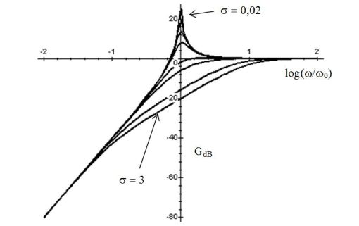
The following figures give the Bode diagram in gain and phase of a band pass filter \(2nd\) order. Different numerical values of \(\sigma\) are used.
Fondamental : The terminals L open output : high - pass filter
The voltage divider rule gives :
\(\underline H (j\omega ) = \frac{{jL\omega }}{{R + \;jL\omega + \frac{1}{{jC\omega }}}} = \frac{{ - LC{\omega ^2}}}{{1 - LC{\omega ^2} + jRC\omega \;}}\)
We want to write this transfer function in the standard form :
\(\underline H (j\omega ) = \frac{{\left( { - \frac{{{\omega ^2}}}{{\omega _0^2}}} \right)}}{{1 - \frac{{{\omega ^2}}}{{\omega _0^2}} + 2j\sigma \frac{\omega }{{{\omega _0}}}}}K\)
For identification, we find the same characteristics as for the low-pass and band-pass filters :
\({\omega _0} = \frac{1}{{\sqrt {LC} }}\;\;\;\;\;;\;\;\;\;\;\sigma = \frac{1}{2}RC{\omega _0} = \frac{R}{2}\sqrt {\frac{C}{L}} \;\;\;\;\;;\;\;\;\;\;K = 1\)
So :
\(\underline H (j\omega ) = \frac{{\left( { - \frac{{{\omega ^2}}}{{\omega _0^2}}} \right)}}{{1 - \frac{{{\omega ^2}}}{{\omega _0^2}} + 2j\sigma \frac{\omega }{{{\omega _0}}}}}\;\;\;\;\;\;\;so\;\;\;\;\;\;\;\left\{ \begin{array}{l}G(\omega ) = \frac{{\left( {\frac{{{\omega ^2}}}{{\omega _0^2}}} \right)}}{{\sqrt {{{\left( {1 - \frac{{{\omega ^2}}}{{\omega _0^2}}} \right)}^2} + 4{\sigma ^2}{{\left( {\frac{\omega }{{{\omega _0}}}} \right)}^2}} }} \\{\varphi _{high-pass}} = {\varphi _{low-pass}} + \pi \\\end{array} \right.\)
The following figures give the Bode diagram in gain and phase of a high-pass filter \(2nd\) order. Different numerical values of \(\sigma\) are used.

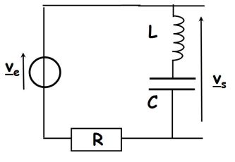
Fondamental : The terminals of (C + L) output open: notch or band - stop filter
The voltage divider rule gives :
\(\underline H (j\omega ) = \frac{{\frac{1}{{jC\omega }} + jL\omega \;}}{{R + jL\omega \; + \frac{1}{{jC\omega }}}} = \frac{{1 - LC{\omega ^2}}}{{1 - LC{\omega ^2} + jRC\omega \;}}\)
We want to write this transfer function in the standard form :
\(\underline H (j\omega ) = \frac{{1 - \frac{{{\omega ^2}}}{{\omega _0^2}}}}{{1 - \frac{{{\omega ^2}}}{{\omega _0^2}} + 2j\sigma \frac{\omega }{{{\omega _0}}}}}K\)
For identification, we find the same characteristics as for the low-pass, band-pass and high-pass filters :
\({\omega _0} = \frac{1}{{\sqrt {LC} }}\;\;\;\;\;;\;\;\;\;\;\sigma = \frac{1}{2}RC{\omega _0} = \frac{R}{2}\sqrt {\frac{C}{L}} \;\;\;\;\;;\;\;\;\;\;K = 1\)
So :
\(\underline H (j\omega ) = \frac{{1 - \frac{{{\omega ^2}}}{{\omega _0^2}}}}{{1 - \frac{{{\omega ^2}}}{{\omega _0^2}} + 2j\sigma \frac{\omega }{{{\omega _0}}}}} = \frac{1}{{1 + \frac{{2j\sigma }}{{\left( {\frac{{{\omega _0}}}{\omega } - \frac{\omega }{\omega }} \right)}}}}\;\;\;\;\;\;\;so\;\;\;\;\;\;\;\left\{ \begin{array}{l}G(\omega ) = \frac{1}{{\sqrt {1 + \frac{{4{\sigma ^2}}}{{{{\left( {\frac{{{\omega _0}}}{\omega } - \frac{\omega }{\omega }} \right)}^2}}}} }} \\{\varphi _{band-stop}} = {\varphi _{low-pass}} \pm \pi \\\end{array} \right.\)
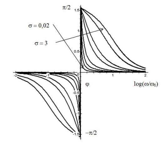
The following figures give the Bode diagram in gain and phase of a notch filter \(2nd\) order. Different numerical values of \(\sigma\) are used.