Magnetic energy of a two-circuits system
Fondamental : Ohm's generalized law
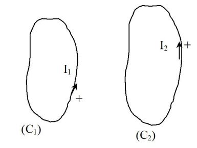
Two wire circuits \((C_1)\) and \((C_2)\) are in mutual coupling.
So in the absence of other sources of magnetic field :
\({\Phi _1} = {L_1}{I_1} + M{I_2}\;\;\;\;\;\;\;and\;\;\;\;\;\;\;{\Phi _2} = {L_2}{I_2} + M{I_1}\)
\(\Phi_1\) is the total magnetic flux through the circuit \((C_1)\) and \(\Phi_2\) the total magnetic flux through the circuit \((C_2)\).
If the two circuits are rigid and still in the laboratory referential, the inductive electromotive forces are :
\({e_1} = - \frac{{d{\Phi _1}}}{{dt}} = - {L_1}\frac{{d{I_1}}}{{dt}} - M\frac{{d{I_2}}}{{dt}}\;\;\;\;\;\;\;and\;\;\;\;\;\;\;{e_2} = - \frac{{d{\Phi _2}}}{{dt}} = - {L_2}\frac{{d{I_2}}}{{dt}} - M\frac{{d{I_1}}}{{dt}}\)
The voltage differences between the frames of each circuit are :
\({u_1} = {R_1}{I_1} - {e_1} = {R_1}{I_1} + {L_1}\frac{{d{I_1}}}{{dt}} + M\frac{{d{I_2}}}{{dt}}\;\;\;\;\;\;\;and\;\;\;\;\;\;\;{u_2} = {R_2}{I_2} - {e_2} = {R_2}{I_2} + {L_2}\frac{{d{I_2}}}{{dt}} + M\frac{{d{I_1}}}{{dt}}\)
Fondamental : Magnetic energy of the two-circuits system
The electric power received by the two circuits is :
\(P = {u_1}{I_1} + {u_2}{I_2}\)
So :
\(P = \left( {{R_1}{I_1}^2 + \frac{d}{{dt}}\left( {\frac{1}{2}{L_1}{I_1}^2} \right) + M{I_1}\frac{{d{I_2}}}{{dt}}} \right) + \left( {{R_2}{I_2}^2 + \frac{d}{{dt}}\left( {\frac{1}{2}{L_2}{I_2}^2} \right) + M{I_2}\frac{{d{I_1}}}{{dt}}} \right)\)
\(P = {R_1}{I_1}^2 + {R_2}{I_2}^2 + \frac{d}{{dt}}\left( {\frac{1}{2}{L_1}{I_1}^2} \right) + \frac{d}{{dt}}\left( {\frac{1}{2}{L_2}{I_2}^2} \right) + M\frac{d}{{dt}}({I_1}{I_2})\)
Finally :
\(P = ({R_1}{I_1}^2 + {R_2}{I_2}^2) + \frac{d}{{dt}}\left( {\frac{1}{2}{L_1}{I_1}^2 + \frac{1}{2}{L_2}{I_2}^2 + M{I_1}{I_2}} \right)\)
The power dissipated by Joule effect can be recognized :
\(P_{Joule}={R_1}{I_1}^2 + {R_2}{I_2}^2\)
Another energy can be defined :
\({E_m} = \frac{1}{2}{L_1}{I_1}^2 + \frac{1}{2}{L_2}{I_2}^2 + M{I_1}{I_2}\)
This is the magnetic energy of the two-circuits system, in the absence of other sources of magnetic field.
The convention used is that this energy is equal to zero when the currents are equal to zero.
Attention : Energy of the two circuits system
\({E_m} = \frac{1}{2}{L_1}{I_1}^2 + \frac{1}{2}{L_2}{I_2}^2 + M{I_1}{I_2}\)
Remarque : Ideal coupling
It is proven that :
\(\left| M \right| \le \sqrt {{L_1}{L_2}}\)
We define :
\(k = \frac{{\left| M \right|}}{{\sqrt {{L_1}{L_2}} }}\)
\(k\) defines the coupling coefficient between the two circuits.
This coefficient has a value ranged between \(0\) and \(1\).
The case \(k=1\), or \(\left| M \right| = \sqrt {{L_1}{L_2}}\), corresponds to the situation where all the magnetic field lines created by one of the two circuits cross the other circuit.
It is the ideal case of perfect coupling.
Exemple : Exercises on coupled circuits
Consider this circuit :
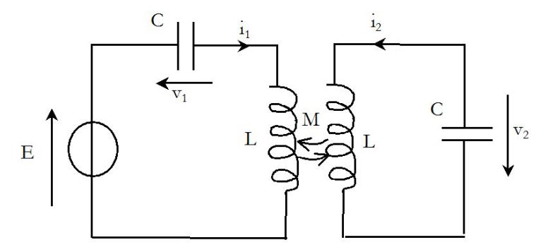
Intensities and voltages are linked :
\({i_1} = C\frac{{d{v_1}}}{{dt}}\;\;\;\;\;\;\;and\;\;\;\;\;\;\;{i_2} = C\frac{{d{v_2}}}{{dt}}\)
\(E = {v_1} + L\frac{{d{i_1}}}{{dt}} + M\frac{{d{i_2}}}{{dt}}\;\;\;\;\;\;\;and\;\;\;\;\;\;\;{v_2} + L\frac{{d{i_2}}}{{dt}} + M\frac{{d{i_1}}}{{dt}} = 0\)
Hence :
\(\left\{ \begin{array}{l}E = {v_1} + LC\frac{{{d^2}{v_1}}}{{d{t^2}}} + MC\frac{{{d^2}{v_2}}}{{d{t^2}}} \\{v_2} + LC\frac{{{d^2}{v_2}}}{{d{t^2}}} + MC\frac{{{d^2}{v_1}}}{{d{t^2}}} = 0 \\\end{array} \right.\)
Proper modes research :
Suppose \(E=0\) (free running).
The solutions researched are harmonic and of same pulsation \(\omega\).
So :
\(0 = {v_1} - LC{\omega ^2}{v_1} - MC{\omega ^2}{v_2}\;\;\;\;\;\;\;and\;\;\;\;\;\;\;{v_2} - LC{\omega ^2}{v_2} - MC{\omega ^2}{v_1} = 0\)
Hence the homogenous system :
\((1 - LC{\omega ^2}){v_1} - MC{\omega ^2}{v_2} = 0\;\;\;\;\;\;\;and\;\;\;\;\;\;\; - MC{\omega ^2}{v_1} + (1 - LC{\omega ^2}){v_2} = 0\)
This system has one non trivial solution if its determinant is equal to zero :
\({(1 - LC{\omega ^2})^2} - {(MC{\omega ^2})^2} = 0\)
So :
\((1 - LC{\omega ^2} - MC{\omega ^2})(1 - LC{\omega ^2} + MC{\omega ^2}) = 0\)
Hence the two own pulses (with \(M<L\)) :
\({\omega _1} = \frac{1}{{\sqrt {(L + M)C} }}\;\;\;\;\;\;\;\;\;\;and\;\;\;\;\;\;\;\;\;\;{\omega _2} = \frac{1}{{\sqrt {(L - M)C} }}\)
For the first proper mode, \(v_1=v_2\) : the two voltages oscillate in accordance.
For the second proper mode, \(v_1=-v_2\) : the two voltages oscillate in opposite accordance.
The free running corresponds to the linear addition of these two proper modes.
Remarque : Another definition of self-inductance of a circuit
The circuit is a wire loop (or not) without any interaction with another circuit.
To expand the definition of \(L\), we can identify the two expressions of the magnetic energy, hence :
\(\frac{1}{2}L{I^2} = \iiint_{(V)}\frac{{B_{propre}^2}}{{2{\mu _0}}}d\tau\)