In the further course, we will suppose that the temperature imbalances (responsible for the heat transfers) are weak.

So, we will always be able to define at each point \(M\) and each moment \(t\) a temperature, a pression, a density... (“local thermodynamic balance” axiom).

The presence, in the macroscopically motionless material medium, of a temperature inhomogeneity creates a conductive thermal transfer, that has the following properties :

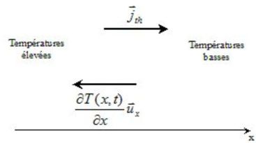
• The transfer is made from the hottest zones to the coldest ones.

• It is proportionnal to the surface through which we evaluate the power scattered, and also proportional to the duration of the transfer.

• It grows linearly with the temperature gradient.

Joseph Fourier (1768 – 1830) introduced a phenomenological law to describe this conductive heat transfer.

Let's consider a body with a temperature that only depends on \(x\) and on the time \(t\).

The energy quantity \(\delta Q\) that goes by thermal conduction through an elementary surface \(dS\), perpendicular to the \((Ox)\) axis during \(dt\), in the chosen direction for \((Ox)\) is :

\(\delta Q = - \lambda \frac{{\partial T(x,t)}}{{\partial x}}dS\ dt\)

where \(\lambda\) (sometimes noted \(K\)) is a positive constant, typical of the material, called thermal conductivity (in \(W.m^{-1}.K^{-1}\)).

We define the thermal current density vector : (by analogy with the electric current density vector)

\({j_{th}} = \frac{{\delta Q}}{{dSdt}} = - \lambda \;\frac{{\partial T(x,t)}}{{\partial x}}\)

Or :

\({\vec j_{th}} = {j_{th}}{\vec u_x} = - \lambda \frac{{\partial T(x,t)}}{{\partial x}}{\vec u_x} = - \lambda\; \overrightarrow {grad} \;T(x,t)\)

The last expression, in which the temperature gradient is displayed, is Fourier's law.

It is generalized into a three-dimensional law :

\({\vec j_{th}} = - \lambda \;\overrightarrow {grad} \ T(x,y,z,t) = - \lambda \left( {\frac{{\partial T(x,y,z,t)}}{{\partial x}}{{\vec u}_x} + \frac{{\partial T(x,y,z,t)}}{{\partial y}}{{\vec u}_y} + \frac{{\partial T(x,y,z,t)}}{{\partial z}}{{\vec u}_z}} \right)\)

The quantity :

\(\frac{{\delta Q}}{{dt}} = {j_{th}}.dS = {\vec j_{th}}.dS\;{\vec u_x}\)

is the thermal flow noted \(P\) (it is a thermal power) : it can be interpreted as the flux of \({\vec j_{th}}\)  through the oriented surface \(dS\) (equivalent to the electric current).

The conductivities \(\lambda\) are in \(W.m^{-1}.K^{-1}\) :

• Gas (\(\lambda\) from \(0,006\) to \(0,18\)) : conducts poorly

• Non-metal liquids (\(\lambda\) from \(0,1\) to \(1\)) : normal conductors

• Metals (\(\lambda\) from \(10\) to \(400\)) : excellent conductors (copper, steel)

• Non-metal materials (\(\lambda\) from \(0,004\) to \(4\)) : normal conductors (glass, concrete, wood) or bad ones (glass wool, expanded polystyrene)