A few classical applications
Fondamental : Damped harmonic oscillator
The motion of a damped harmonic oscillator follows the following (one dimensional) equation :
\(m\ddot x = - kx - hm\dot x\;\;\;\;\;soit\;\;\;\;\;\ddot x + h\dot x + \frac{k}{m}x = 0\)
We note :
\({\omega _0} = \sqrt {\frac{k}{m}} \;\;\;\;\;;\;\;\;\;\;h = 2\lambda = 2\sigma {\omega _0} = \frac{{{\omega _0}}}{Q}\)
\(\sigma\) is the damping ratio and \(Q\) the quality factor :
\(Q=\frac {1}{2\sigma}\)
Then :
\(\;\ddot x + 2\lambda \dot x + \omega _0^2x = \ddot x + 2\sigma {\omega _0}\dot x + \omega _0^2x = \ddot x + \frac{{{\omega _0}}}{Q}\dot x + \omega _0^2x = 0\)
We look for solutions like \(exp(rt)\), with \(r\) a complex number.
The characteristic equation is :
\(r^2+2\sigma \omega_0 r+\omega_0^2=0\)
The discriminant is :
\(\Delta=4\omega_0^2(\sigma^2-1)\)
Different types of solution are observed : it depends on the value of \(\sigma\) (or \(Q=1/2\sigma\)) :
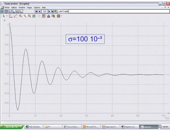
Underdamping : (if \(\sigma<1\))
If \(x(0)=x_0\) and if the initial velocity is equal to zero :
\(\begin{array}{l}x(t) = {x_0}{e^{ - \sigma {\omega _0}t}}\left( {\cos (\omega t) + \frac{{\sigma {\omega _0}}}{\omega }\sin (\omega t)} \right) \\x(t) = C{e^{ - \sigma {\omega _0}t}}\cos (\omega t - \phi ) \\C = x_0^{}\sqrt {1 + {{\left( {\frac{{\sigma {\omega _0}}}{\omega }} \right)}^2}} \;\;\;;\;\;\;\tan \phi = \frac{{\sigma {\omega _0}}}{\omega } \\\end{array}\)
With :
\(\omega = {\omega _0}\sqrt {1 - {\sigma ^2}} \)
The undamped angular frequency.
The \(Q\)-factor gives the order of magnitude of the number of oscillations we can experimentally measure.
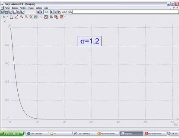
Overdamping : (so \(\sigma>1\))
If \(x(0)=x_0\) and if the initial velocity is equal to zero :
\({r_1} = - \sigma {\omega _0} + {\omega _0}\sqrt {{\sigma ^2} - 1} \;;\;{r_2} = - \sigma {\omega _0} - {\omega _0}\sqrt {{\sigma ^2} - 1}\)
\(\begin{array}{l}\omega = {\omega _0}\sqrt {{\sigma ^2} - 1} \\x(t) = {x_0}{e^{ - \sigma {\omega _0}t}}\left( {ch(\omega t) + \frac{{\sigma {\omega _0}}}{\omega }sh(\omega t)} \right) \\x(t) = \frac{{{x_0}}}{2}{e^{ - \sigma {\omega _0}t}}\left( {\left( {1 - \frac{{\sigma {\omega _0}}}{\omega }} \right){e^{ - \omega t}} + \left( {1 + \frac{{\sigma {\omega _0}}}{\omega }} \right){e^{\omega t}}} \right) \\\end{array}\)
Critical damping : (then \(\sigma=1\))
If \(x(0)=x_0\) and if the initial velocity is equal to zero :
\(x(t) = {x_0}(1 + {\omega _0}t){e^{ - {\omega _0}t}}\)
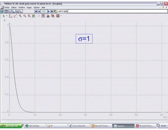
Underdamping and Overdamping

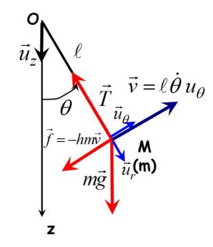
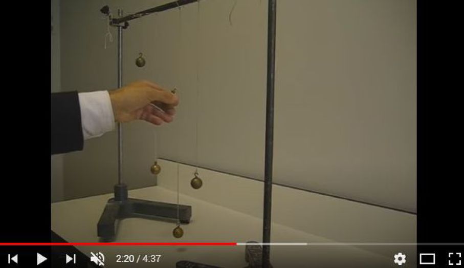
Fondamental : Simple pendulum
If there is a viscous friction force :
\(\vec f_v=-hm\vec v\)
The second law of motion projected on \(\vec u_{\theta}\) gives (the equivalent of the second law for angular momentum can be used as well) :
\(m\ell \ddot \theta = - mg\sin \theta - hm(\ell \dot \theta )\)
It follows :
\(\ddot \theta + h\dot \theta + \frac{g}{\ell }\sin \theta = \ddot \theta + 2\sigma {\omega _0}\dot \theta + \omega _0^2\sin \theta = 0\)
If the angle \(\theta\) is « small », the usual equation appears :
\(\ddot \theta + h\dot \theta + \frac{g}{\ell }\theta = \ddot \theta + 2\sigma {\omega _0}\dot \theta + \omega _0^2\theta = 0\)

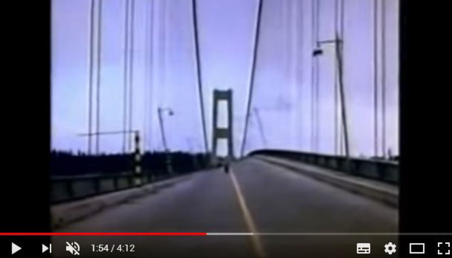
Exemple : An impressive mechanical resonance : the Tacoma bridge resounding
Fondamental : Sinusoidally driven mechanical oscillators
Why is this study useful ?
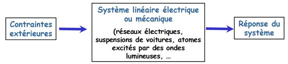
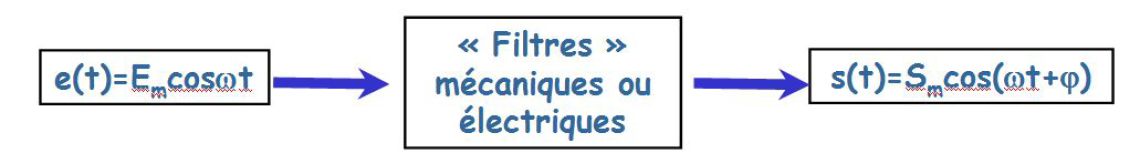
Harmonic analysis is the study of the output \(s(t)\) of a system when the input is a sinusoidal signal \(e(t)\) with variable driving angular frequency \(\omega\).
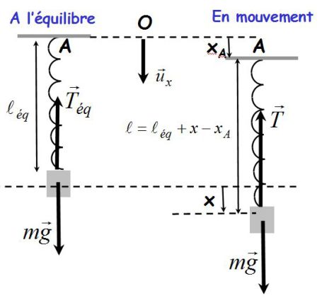
Chosen model : vertical mechanical oscillator with movable attached point.
The attached point is in A (see figure).
In the inertial reference frame of the Earth :
\(m\ddot x = mg - hm\dot x - k({\ell _{eq}} + x - {x_A} - {\ell _0})\)
Equilibrium condition :
\(\ddot x + h\dot x + \frac{k}{m}x = \frac{k}{m}{x_A}\)
With the usual notations :
\(\ddot x + 2\sigma {\omega _0}\dot x + \omega _0^2x = \omega _0^2{x_A}\)
In what follows, we suppose :
\({x_A} = {X_{A,m}}\cos (\omega t)\)
This equation is equivalent to the one giving the tension of a capacitor in a RLC circuit (see electrokinetic course).
If \(u_C\) is the tension of the capacitor : (\(u_C=q/C\))
\(L\ddot q + R\dot q + \frac{1}{C}q = e(t)\)
So :
\({\ddot u_C} + \frac{R}{L}{u_C} + \frac{1}{{LC}}{u_C} = \frac{1}{{LC}}e(t)\)
Resolution with complex numbers (the same as in electricity) :
We note :
\({\underline x _A} = {X_{A,m}}{e^{i\omega t}}\;\;\;\;\;;\;\;\;\;\;\;\;\underline x = {X_m}{e^{i(\omega t + \phi )}}\;\;\;(x = {X_m}\cos (\omega t + \phi ))\)
Then :
\(\underline {\dot x} = i\omega \underline x \;\;\;\;\;\;\;\;\;\;and\;\;\;\;\;\;\;\;\;\;\underline {\ddot x} = i\omega \underline {\dot x} = {(i\omega )^2}\underline x = - {\omega ^2}\underline x\)
Output \(x(t)\) :
\(\begin{array}{l}\ddot x + 2\sigma {\omega _0}\dot x + \omega _0^2x = \omega _0^2{x_A} \\- \omega _{}^2\underline x + 2\sigma {\omega _0}(i\omega \underline x ) + \omega _0^2\underline x = \omega _0^2{\underline x _A} \\\left[ {(\omega _0^2 - \omega _{}^2) + 2i\sigma {\omega _0}\omega } \right]\;\underline x = \omega _0^2{\underline x _A} \\\end{array}\)
Then :
\(\;\underline x = \frac{{\omega _0^2}}{{(\omega _0^2 - \omega _{}^2) + 2i\sigma {\omega _0}\omega }}{\underline x _A}\)
Or :
\({X_m}{e^{i\phi }} = \frac{{\omega _0^2}}{{(\omega _0^2 - \omega _{}^2) + 2i\sigma {\omega _0}\omega }}{X_{A,m}}\)
The maximum value is the modulus of that expression :
\({X_m} = \frac{{\omega _0^2}}{{\sqrt {{{(\omega _0^2 - \omega _{}^2)}^2} + 4{\sigma ^2}\omega _0^2{\omega ^2}} }}{X_{A,m}}\)
\(X_m\) is maximum for an angular frequency (which exists only if \(\sigma <1/\sqrt{2}\)) :
\(\;\omega _r^{} = \omega _0^{}\sqrt {1 - 2{\sigma ^2}}\)
And the maximum value is :
\({X_m}({\omega _r}) = \frac{1}{{2\sigma \sqrt {1 - {\sigma ^2}} }}{X_{A,m}}\)
By using the \(Q\)-factor instead of the damping ratio \(\sigma\) :
\(\;\omega _r^{} = \omega _0^{}\sqrt {1 - \frac{1}{{2{Q^2}}}} \;\;\;\;\;\;\;\;\;\;with\;\;\;\;\;\;\;\;\;\;Q > \frac{1}{{\sqrt 2 }}\)
And :
\({X_m}({\omega _r}) = \frac{Q}{{\sqrt {1 - \frac{1}{{4{Q^2}}}} }}{X_{A,m}}\)
Note :
If the damping is small (\(\sigma\) "small" and \(Q\) "large"), then :
\(\;\omega _r^{} \approx \omega _0^{}\;\;\;\;\;and\;\;\;\;\;{X_m}({\omega _r}) \approx Q{X_{A,m}}\)
If \(Q=10\), the amplitude of the resonance is \(10\) times the one of the input signal : the resonance is « acute » and can cause the destruction of the oscillating system.
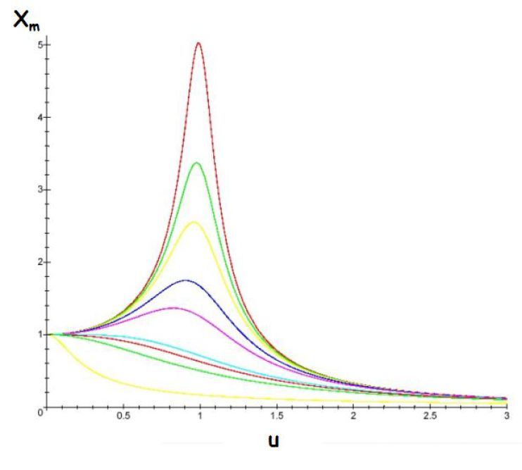
The previous figure gives the output \(X_m(\omega)\) for different values of the \(Q\)-factor.
We chose \(X_{A,m}=1\) and \(u=\omega/\omega_0\).
The larger the \(Q\)-factor, the more acute the resonance becomes.
The oscillator is low-pass filter, with or without resonance.
Speed output :
If \(v\) is real : \(v(t) = {V_m}\cos (\omega t + \psi )\)
If \(v\) is complex : : \(\underline v (t) = {V_m}{e^{i(\omega t + \psi )}}\)
We note that \(\underline v = \underline {\dot x} = i\omega x\). It follows :
\(\;\underline v = i\omega \left( {\frac{{\omega _0^2}}{{(\omega _0^2 - \omega _{}^2) + 2i\sigma {\omega _0}\omega }}{{\underline x }_A}} \right) = \frac{{{\omega _0}}}{{i\left( {\frac{\omega }{{{\omega _0}}} - \frac{{{\omega _0}}}{\omega }} \right) + 2\sigma }}{\underline x _A}\)
Or :
\({V_m}{e^{i\psi }} = \frac{{\omega _0^{}}}{{2\sigma + i\left( {\frac{\omega }{{{\omega _0}}} - \frac{{{\omega _0}}}{\omega }} \right)}}{X_{A,m}}\)
The maximum amplitude \(V_m(\omega)\) is given by the modulus :
\({V_m}(\omega ) = \frac{{\omega _0^{}}}{{\sqrt {4{\sigma ^2} + {{\left( {\frac{\omega }{{{\omega _0}}} - \frac{{{\omega _0}}}{\omega }} \right)}^2}} }}{X_{A,m}}\)
\(V_m(\omega)\) is maximum (velocity resonance) if the denominator is minimum, for an angular frequency :
\(\frac{\omega }{{{\omega _0}}} - \frac{{{\omega _0}}}{\omega } = 0\;\;\;\;\;\;\;\;\;\;\;so\;\;\;\;\;\;\;\;\;\;\;\omega = {\omega _0}\)
The amplitude of the velocity is :
\({V_m}({\omega _0}) = \frac{{\omega _0^{}}}{{2\sigma }}{X_{A,m}} = Q\omega _0^{}{X_{A,m}}\)
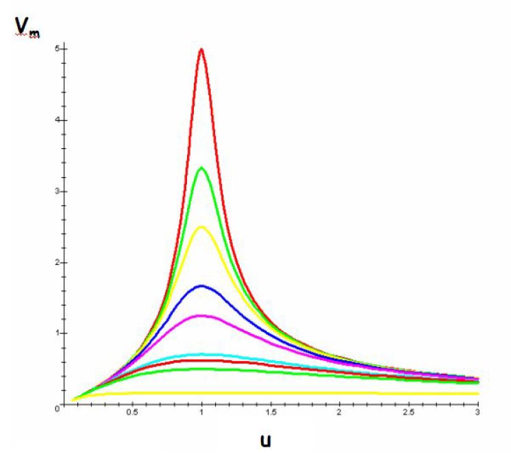
The previous figure gives \(V_m(\omega)\) for different values of the \(Q\)-factor.
We chose \(X_{A,m}=1\) and \(u=\omega/\omega_0\).
The larger the \(Q\)-factor, the more acute the resonance becomes.
The oscillator is a band-pass filter.
Bandwidth of this band-pass filter :
An angular frequency is in the bandwidth if the output gain is, by definition, superior to the maximal gain (which we obtain when \(\omega_0\) is plugged in) divided by \(\sqrt{2}\).
The bandwidth length is :
\(\Delta \omega = {\omega _{{c_2}}} - {\omega _{{c_1}}} = 2\sigma {\omega _0} = \frac{{{\omega _0}}}{Q}\)
The smaller it is (acute resonance), the smaller the damping gets (and the larger the \(Q\)-factor becomes).