Gauss' law
Presentation of electricity and magnetism video (Référence : "Physique collégiale")

Fondamental :
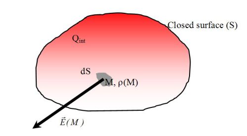
From the Maxwell-Gauss equation, we can calculate the flux of the electric field exiting through a closed surface \((S)\) :
\( \oint_S\vec {E}.\vec{n} \ dS=\iiint_{V} div\vec{E} \ d\tau=\frac{1}{\epsilon_0}\iiint_{V} \rho \ d\tau=\frac{1}{\epsilon_0}Q_{int}\)
Where \(Q_{int}\) represents the charges inside the closed surface \((S)\).
Gauss' law is still true in a time-depending regime, even though the electric charges can be moving.
In steady-state, the sources of the electric field are the charges characterized by their density \(\rho\).
The field lines diverge from positive charges like a fluid coming out of a true source. They disappear on negative charges like a fluid in a well.
It is still true in a non steady-state, although \(\rho\) is not the only source of electric field anymore. Thus electric field maps are not necessarily similar (See the consequence of the Maxwell-Faraday equation).
Attention : Gauss' law
\( \oint_S\vec {E}.\vec{n} \ dS=\frac{1}{\epsilon_0}Q_{int}\)
Complément : Gauss' law for the gravitationnal field
We can observe the formal analogy between the electric Coulomb field created by a punctual charge :
\(\vec E = \frac{1}{{4\pi \varepsilon _0 }}q\frac{{\overrightarrow {OM} }}{{OM^3 }}\)
And the Newton gravitational field \(\vec g\) created by a punctual mass :
\(\vec g = - Gm\frac{{\overrightarrow {OM} }}{{OM^3 }}\)
\(G\) represents the universal gravitational constant.
We can then associate the charge \(q\) to the mass \(m\) and the constant \(\ \frac{1}{{\varepsilon _0 }}\) to \(-4\pi G\).
Thus, Gauss' law remains true for the integral form of the gravitational field \(\vec g\) :
\(\oint_S\vec {g}.\vec{n} \ dS=-4\pi Gm_{int}\)
And its local form :
\(div\vec g = - 4\pi G\rho \)
Where \(\rho\) is the density at M, the point considered.
Attention : Gauss' law for the gravitationnal field
\(\oint_S\vec {g}.\vec{n} \ dS=-4\pi Gm_{int}\)
And its local form :
\(div\vec g = - 4\pi G\rho \)
Méthode : Classic uses of Gauss' law
In highly symmetrical problems, Gauss' law is an easy way to compute the electric field. It is useful in these classic situations and must be remembered.
Infinite plane evenly charged in surface (with constante \(\sigma\)) :
\(\vec E=+ \frac{\sigma}{2\varepsilon_0}\vec u_z\) above the plane and \(\vec E=- \frac{\sigma}{2\varepsilon_0}\vec u_z\) below the plane
Where (Oz) is perpendicular to the charged plane.
Sphere of center O and radius equal to R, charged in volume (\(\rho = cste\) and \(Q\) is the total charge, \(Q=\frac{4}{3}\pi R^3 \rho\)) :
If \(r>R\) : \(\vec E(M)=\frac{Q}{4\pi\varepsilon_0}\frac{\vec u_r}{r^2}\)
If \(r<R\) : \(\vec E(M)=\frac{Q}{4\pi\varepsilon_0}\frac{r}{R^3}\vec u_r\)
Here the spherical base is used.

Infinite wire linearly charged (\(\lambda = cste\)) :
\(\vec E(M)=\frac {\lambda}{2\pi\varepsilon_0}\frac{\vec u_r}{r}\)
Here the cylindrical base is used.