Electrostatic dipole
Définition : Electrostatic dipole
A rigid set of two punctual charges \(+q\) and \(-q\) (globally neutral) at the distance \(2a\) from each other is called an “electrostatic diplole”.
Such a model can explain :
Polar molecules (for instance : HCl, H2O)
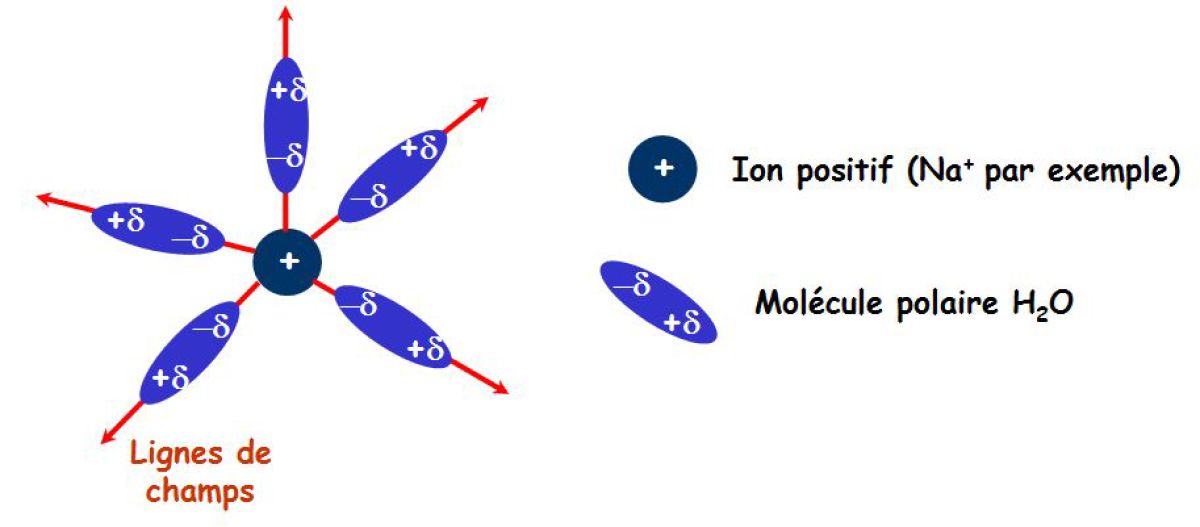
Atom polarization in an exterior electric field (solvation of ions phenomenon)
Fondamental : Determination of the potential created by the dipole
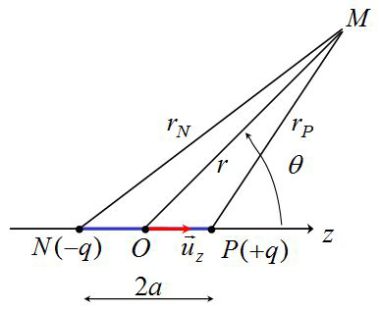
We calculate the potential created by the dipole located in a point M in space.
Revolution symmetry around (Oz) axis : we choose \(M(r,\theta)\) in the plane of the two charges.
Under the dipole approximation \(r>>a\) (we study the charges from « far » away, i.e. at a distance greatly superior to a few \(nm\)).
The potential in the point M is (superposition principle) :
\(V(M) = \frac{1}{{4\pi {\varepsilon _0}}}\frac{q}{{{r_P}}} - \frac{1}{{4\pi {\varepsilon _0}}}\frac{q}{{{r_N}}} = \frac{1}{{4\pi {\varepsilon _0}}}q\left( {\frac{1}{{{r_P}}} - \frac{1}{{{r_N}}}} \right)\)
(With : \({r_P} = PM\;and\;{r_N} = NM\; > > \;a\))
According to the Chasles relation :
\(\overrightarrow {PM} = \overrightarrow {OM} - \overrightarrow {OP} = \vec r - a\;{\vec u_z}\)
The squared value :
\(P{M^2} = {r^2} + {a^2} - 2\vec r.a\;{{\vec u}_z}\;\;\;\;\;so\;\;\;\;\;r_P^2 = {r^2} + {a^2} - 2ar\cos \theta\)
Then we compute \(1/r_P\) :
\(\frac{1}{{{r_P}}} = \frac{1}{{\sqrt {{r^2} + {a^2} - 2ar\cos \theta } }} = {\left( {{r^2} + {a^2} - 2ar\cos \theta } \right)^{ - 1/2}}\)
The Taylor expansion until the order \(1\) is :
\({\left( {1 + x} \right)^{ - 1/2}} \approx 1 - \frac{1}{2}x\;\;\;\;\;(x < < 1)\)
Let \(x\) be such as \(x=a/r\) (\(x<<1\)), then :
\(\frac{1}{{{r_P}}} = \frac{1}{r}{\left( {1 + \frac{{{a^2}}}{{{r^2}}} - 2\frac{a}{r}\cos \theta } \right)^{ - 1/2}} \approx \frac{1}{r}\left( {1 + \frac{a}{r}\cos \theta } \right)\)
In the same manner (if \(\theta\) is substituted by \(\pi-\theta\) and \(cos\theta\) by \(-cos\theta\)) :
\(\frac{1}{{{r_N}}} = \frac{1}{r}\left( {1 - \frac{a}{r}\cos \theta } \right)\)
Then :
\(\frac{1}{{{r_P}}} - \frac{1}{{{r_N}}} = 2\frac{a}{{{r^2}}}\cos \theta\)
Thus the potential :
\(V(M) = \frac{1}{{4\pi {\varepsilon _0}}}\frac{{(2aq)}}{{{r^2}}}\cos \theta\)
The dipole moment vector of the electrostatic dipole can be defined by (the vector is oriented from the negative charge to the positive one) :
\(\vec p = (2aq)\;{\vec u_z} = q\overrightarrow {NP}\)
Then (the potential decreases like \(1/r^2\)) :
\(V(M) = \frac{1}{{4\pi {\varepsilon _0}}}\frac{p}{{{r^2}}}\cos \theta\)
By posing \(\vec u_r = \vec r/r\) :
\(V(M) = \frac{1}{{4\pi {\varepsilon _0}}}\frac{{\vec p.{{\vec u}_r}}}{{{r^2}}}\;\;\;\;\;({\vec u_z}.{\vec u_r} = \cos \theta )\)
Définition : Dipole moment vector
The dipole moment vector is a characteristic of the electrostatic dipole.
In the international system of units \(p\) is expressed in \(C.m\).
Yet the Debye unit is more adapted :
\(1\;D = {3,33.10^{ - 30}}C.m\)
Example :
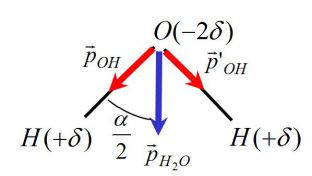
A molecule of water has a dipole moment.
Deduce the charges \(+\delta\) and \(-2\delta\) carried respectively by hydrogen and oxygen atoms.
We know (see figure) :
\(\alpha = (OH,OH) = 104^\circ \;\;\;;\;\;\;\ell = OH = 0,096\;nm\)
The total dipole moment is given by :
\({\vec p_{{H_2}O}} = {\vec p_{OH}} + \vec p{'_{OH}}\)
With :
\({p_{OH}} = p{'_{OH}} = \ell \delta\)
Consequently :
\({p_{{H_2}O}} = 2\ell \delta \cos \frac{\alpha }{2}\)
Thus can be deduced :
\(\delta = \frac{{{p_{{H_2}O}}}}{{2\ell \cos \frac{\alpha }{2}}} \approx \frac{e}{3}\;\;\;\;\;(e = {1,6.10^{ - 19}}C)\)
Méthode : Calculation of the electrostatic field under dipole approximation
The intrinsic relation \(\vec E = - \overrightarrow {grad} \;V\) lets us calculate the field (in polar coordinates) :
\(\left\{ \begin{array}{l}{E_r}(r,\theta ) = - \frac{{\partial V}}{{\partial r}} \\{E_\theta }(r,\theta ) = - \frac{1}{r}\frac{{\partial V}}{{\partial \theta }} \\\end{array} \right.\)
Consequently :
\(\left\{ \begin{array}{l}{E_r} = \frac{1}{{4\pi {\varepsilon _0}}}\frac{{2p\cos \theta }}{{{r^3}}} \\{E_\theta } = \frac{1}{{4\pi {\varepsilon _0}}}\frac{{p\sin \theta }}{{{r^3}}} \\\end{array} \right.\)
Or even :
\(\vec E = \frac{1}{{4\pi {\varepsilon _0}}}\frac{p}{{{r^3}}}\left( {2\cos \theta \;{{\vec u}_r} + \sin \theta \;{{\vec u}_\theta }} \right)\)
Complément : Dipole field topography
Equipotential surface :
The equipotential surface (\(\Sigma_0\)) equation at the potential \(V_0\) is :
\(For\;M\; \in \;({\Sigma _0})\;\;:\;\;V(M) = \frac{1}{{4\pi {\varepsilon _0}}}\frac{p}{{{r^2}}}\cos \theta = {V_0}\)
Thus the equation in polar coordinates :
\({r^2} = A\cos \theta \;\;\;\;\;\;\;\;\;(A = cste)\)
The aspect of equipotential lines is shown on the following picture.
The axis perpendicular to (Oz) and passing through point O is the zero equipotential.
By rotating around (Oz), these lines create equipotential surfaces.
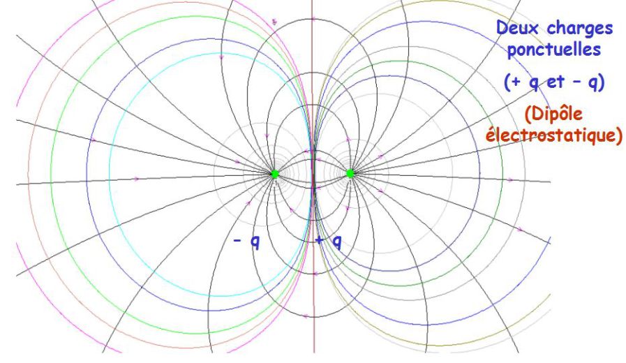
Field lines :
On the field line passing through point M :
\(d\vec r \wedge \vec E = \vec 0\)
Or :
\(\left\{ \begin{array}{l}d\vec r = dr\;{{\vec u}_r} + r\;d\theta \;{{\vec u}_\theta } \\\vec E = {E_r}\;{{\vec u}_r} + {E_\theta }\;{{\vec u}_\theta } \\\end{array} \right.\)
Thus :
\(dr\;{E_\theta } - r\;d\theta \;{E_r} = 0\)
And :
\(\frac{{dr}}{{{E_r}}} = \frac{{r\;d\theta }}{{{E_\theta }}}\)

By replacing the field coordinates by their expressions :
\(\frac{{dr}}{{2\cos \theta }} = \frac{{r\;d\theta }}{{\sin \theta }}\)
Let's separate variables :
\(\frac{{dr}}{r} = 2\frac{{\;\cos \theta }}{{\sin \theta }}d\theta = 2\frac{{\;d(\sin \theta )}}{{\sin \theta }}\)
Then :
\(d(\ln r) = d(\ln (\sin {\theta ^2}))\)
Let \(r\) be \(r=r_0\) for \(\theta=\pi/2\). Then, by integration, we obtain the equation of the field lines in polar coordinates (\(r_0\) is a parameter) :
\(\ln \left( {\frac{r}{{{r_0}}}} \right) = \ln (\sin ^2{\theta})\;\;\;\;\;\;\;so\;\;\;\;\;\;\;r = {r_0}\sin^2 {\theta}\)
The aspect of field lines is given on the previous picture.
Fondamental : Action of an exterior electric field on a dipole
Let an electrostatic dipole be immersed in an electric field \(\vec E_0\) which can be supposed uniform at the dipole scale.
What effect does the field have on the dipole ?
System studied : the (rigid) dipole
Referential of study : laboratory referential (supposed Galilean)
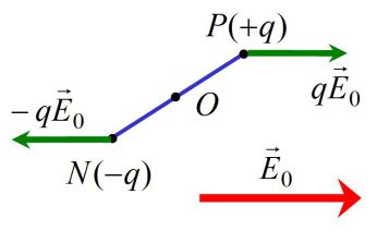
The dipole undergoes two forces \(q \vec E_0\) and \(-q\vec E_0\) which addition is equal to zero.
The dipole undergoes a “force torque”, which moment in relation to O is :
\({\vec M_O} = \overrightarrow {OP} \wedge q{\vec E_0} + \overrightarrow {ON} \wedge ( - q{\vec E_0})\)
Thus :
\({\vec M_O} = (\overrightarrow {OP} - \overrightarrow {ON} ) \wedge q{\vec E_0} = q\overrightarrow {NP} \wedge {\vec E_0}\)
Finally :
\({\vec M_O} = \vec p \wedge {\vec E_0}\)
Under the effect of an electric field, the dipole starts spinning in order to align with the direction of the field (\(\vec p\) and \(\vec E_0\) in the same orientation, stable equilibrium position).
Energetic study :
Let \(V\) be the potential from which the field \(\vec E_0\) ; the potential energy of the (rigid) dipole in this field is :
\({E_p} = qV(P) + ( - q)V(N) = q\left[ {V(P) - V(N)} \right]\)
We remind that \(\vec E_0\) is a gradient field, so :
\(dV=-\vec E . d\vec r\)
Thus, with \(dV=V(P)-V(N)\) :
\(d\vec r = \overrightarrow {OP} - \overrightarrow {ON} = \overrightarrow {NP}\)
Then :
\({E_p} = q( - {\vec E_0}.\overrightarrow {NP} )\)
So :
\({E_p} = - \vec p.{\vec E_0}\)
\(E_p\) is minimum (stable equilibrium position) when \(\vec p\) and \(\vec E_0\) are oriented in the same way.
The following picture illustrates the solvation phenomenon : water molecules align with the field lines created by the charge \(Na^+\).